7.4 The Bayesian Approach to Linear Regression
The Bayesian approach to linear regression is to use a prior distribution for the parameters (coefficient) and then use the data to update the prior distribution to a posterior distribution. It gives us detailed probability about each alternative hypothesis instead of just the null hypothesis. The reasoning about priors for both univariate and multiple regression is based on the Cauchy distribution (looks like a normal distribution with heavier tails). The standardized B- weight, denoted as “beta,” is modeled using the Cauchy distribution. Morey (2012) proposes setting the standard deviation of the Cauchy priors to 1, which corresponds to a prior expectation that beta will typically range from -1 to +1, with values in the centre region close to zero being more frequent (think of a normal distribution centered on 0). Let’s look at the prior distribution for the standardized B-weights:
regOutMCMC <- lmBF(gpa ~ hardwork + basicsmarts + curiosity,
                   data=educdata, posterior=TRUE, iterations=10000)
summary(regOutMCMC)
##
## Iterations = 1:10000
## Thinning interval = 1
## Number of chains = 1
## Sample size per chain = 10000
##
## 1. Empirical mean and standard deviation for each variable,
##    plus standard error of the mean:
##
##               Mean      SD  Naive SE Time-series SE
## mu          0.1621 0.04616 0.0004616      0.0004616
## hardwork    0.5628 0.05073 0.0005073      0.0005161
## basicsmarts 0.5220 0.05003 0.0005003      0.0004971
## curiosity   0.5055 0.04384 0.0004384      0.0004478
## sig2        0.2545 0.03427 0.0003427      0.0003616
## g           1.6716 7.29839 0.0729839      0.0729839
##
## 2. Quantiles for each variable:
##
##                2.5%    25%    50%    75%  97.5%
## mu          0.07282 0.1311 0.1618 0.1930 0.2542
## hardwork    0.46172 0.5293 0.5627 0.5962 0.6641
## basicsmarts 0.42375 0.4890 0.5224 0.5550 0.6198
## curiosity   0.41853 0.4761 0.5053 0.5347 0.5909
## sig2        0.19633 0.2304 0.2515 0.2753 0.3300
## g           0.26580 0.5676 0.9322 1.6316 6.5155
Mean: parameter estimates for the B- weights of each of our predictions sig2: model precision parameter for each iteration that summarizes the error in the model: the smaller sig2, the better the model. We show one of the HDIs by a histogram that shows the posterior distribution of the B-weights for hardwork across all posterior samples.
hist(regOutMCMC[,"hardwork"])
abline(v=quantile(regOutMCMC[,"hardwork"],c(0.025)), col="black")
abline(v=quantile(regOutMCMC[,"hardwork"],c(0.975)), col="black")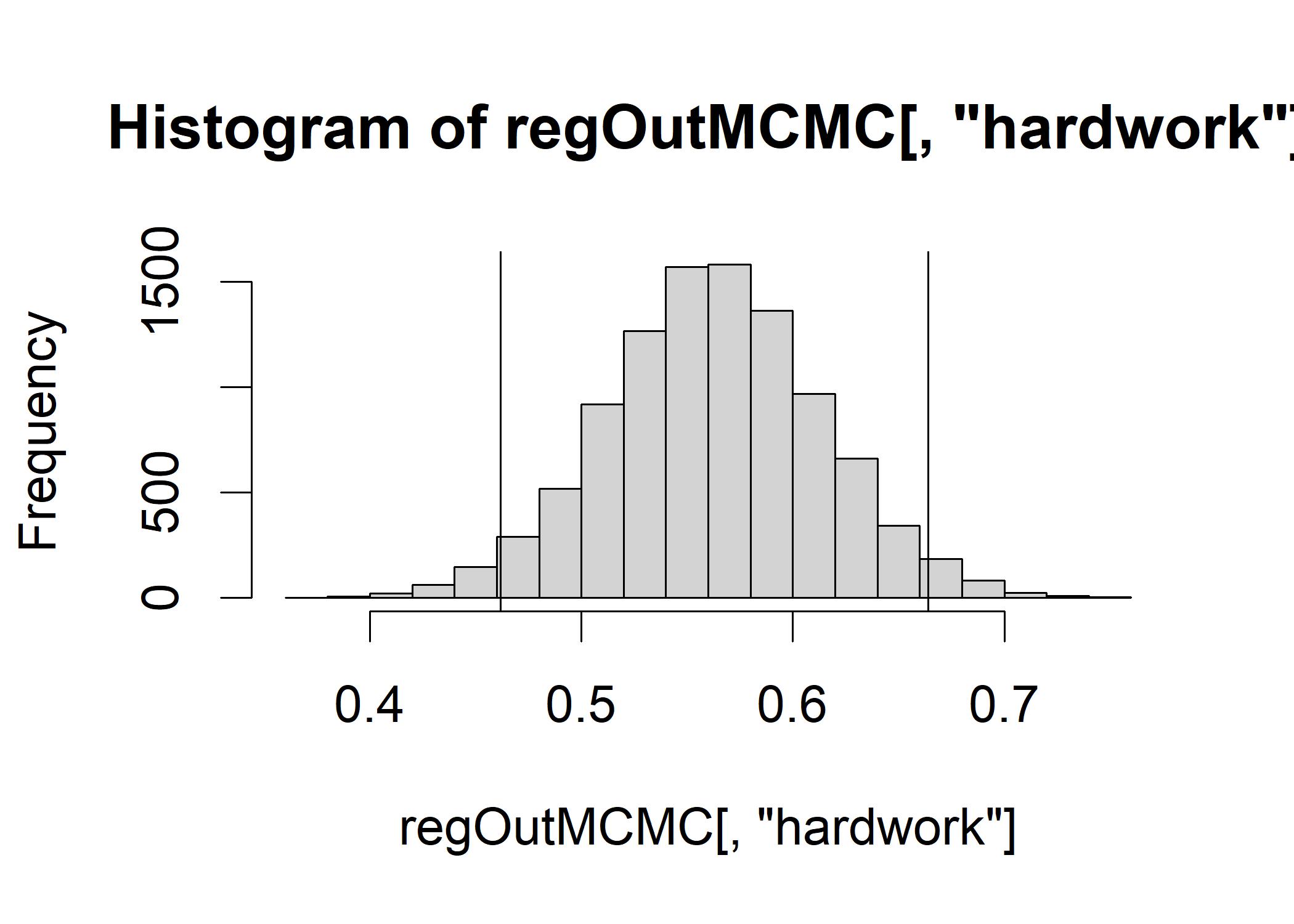 The figure confirms that the posterior distribution of the B-weight for hardwork is centered around 0.56.
In the posterior distribution, the R-squared for each model is given by 1 minus the sig2 value divided by the variance of the dependent variable.
The figure confirms that the posterior distribution of the B-weight for hardwork is centered around 0.56.
In the posterior distribution, the R-squared for each model is given by 1 minus the sig2 value divided by the variance of the dependent variable.
rsqList <- 1 - (regOutMCMC[,"sig2"] / var(gpa))
mean(rsqList) # Overall mean R- squared is 0.75
## [1] 0.7511383
hist(rsqList)
abline(v=quantile(rsqList,c(0.025)), col="black")
abline(v=quantile(rsqList,c(0.975)), col="black")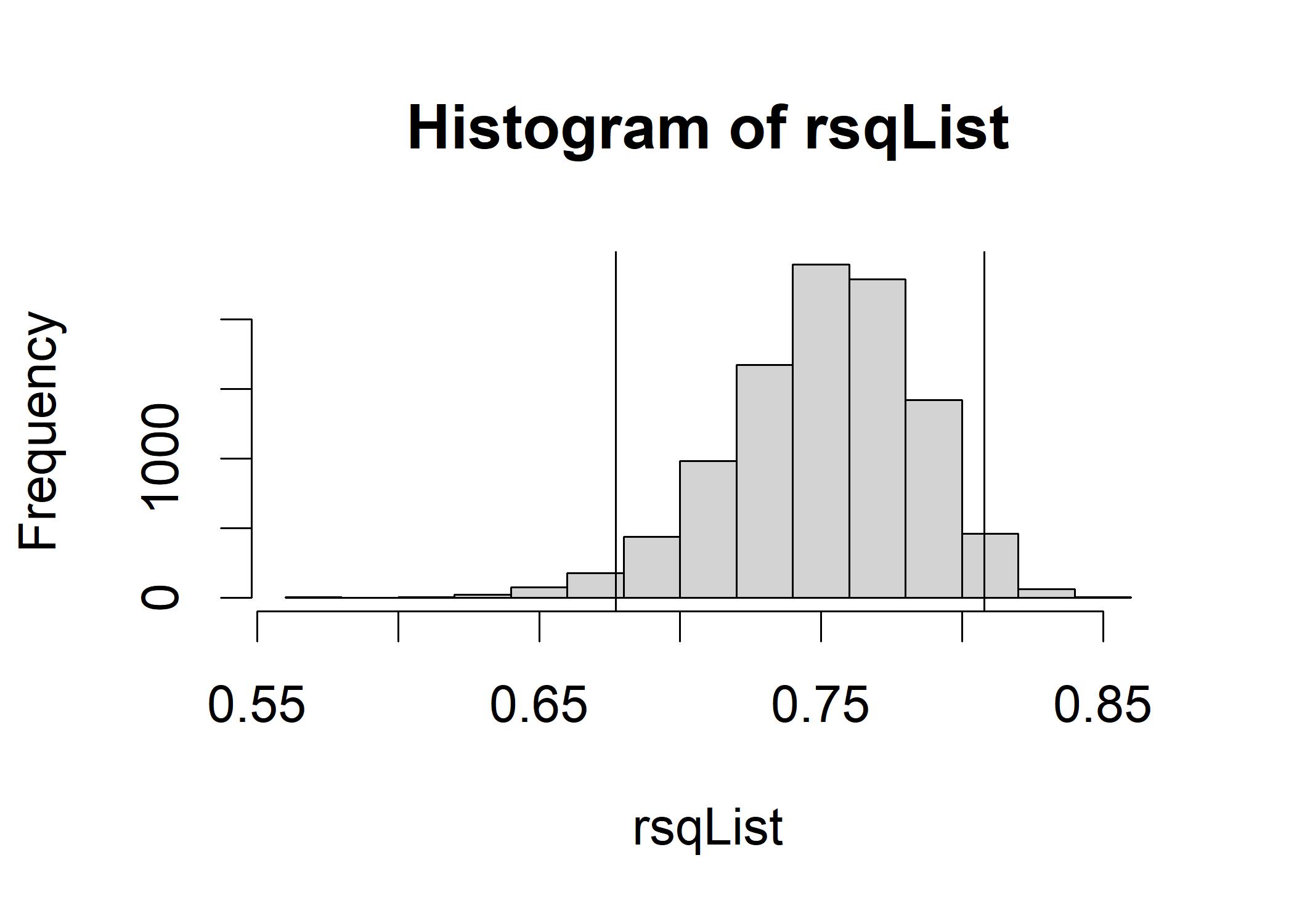 It is reasonable for us to anticipate an R-squared in the underlying population that this sample represents that is as low as about 0.67 or as high as approximately 0.81, with the most likely values of R-squared in that central region surrounding 0.75.
The dependent variable and the predictors (as a set) do not share any variation, as shown by an R-squared value of 0. (The null hypothesis is described in that way.) However, if the R-squared value is 1, the set of predictors correctly predicts the dependent variable.
Finally, we obtain the Bayes factor for the model:
It is reasonable for us to anticipate an R-squared in the underlying population that this sample represents that is as low as about 0.67 or as high as approximately 0.81, with the most likely values of R-squared in that central region surrounding 0.75.
The dependent variable and the predictors (as a set) do not share any variation, as shown by an R-squared value of 0. (The null hypothesis is described in that way.) However, if the R-squared value is 1, the set of predictors correctly predicts the dependent variable.
Finally, we obtain the Bayes factor for the model:
library(BayesFactor)
regOutBF <- lmBF(gpa ~ hardwork + basicsmarts + curiosity, data=educdata)
regOutBF
## Bayes factor analysis
## --------------
## [1] hardwork + basicsmarts + curiosity : 7.885849e+32 ±0%
##
## Against denominator:
##   Intercept only
## ---
## Bayes factor type: BFlinearModel, JZS
In the sense that a model including hardwork, basicsmarts, and curiosity as predictors is greatly preferred over a model that merely has the Y-intercept, the chances are overwhelmingly in favor of the alternative hypothesis (in effect, the Y-intercept- only model means that you are forcing all of the B- weights on the predictors to be 0).