1.1 Descriptive Statistics
Descriptive statistics give us a surface lens through which we can sense the summarized information of the data. They comprise three types of information including 1) measures of central tendency (e.g., mean, median, and mode), 2) measures of dispersion and variability (e.g., range, variance, and standard deviation), and 3) measures of shape (e.g., frequency distribution, skewness and kurtosis).
1.1.1 Measures of Central Tendency
In some scenarios, we would like to know how close each point is to its center point, namely, its central tendency. For instance, we are curious about the central tendency of the age of a sample group. There are several ways the measure the central tendency such as the mean, the median, and the mode, each of which demonstrates different aspects of the central tendency.
Mean
The mean depicts the mathematical central point of a sample of data. Compared to the median and the mode, however, the mean is susceptible to outliers as it will be dragged toward the outliers. Let’s assume we have two groups of people with the ages distribution as follows:
- Age1: [20, 20, 20, 25, 30]
- Age2: [20, 20, 25, 30, 80]
The mean ages of the first group is 27 and that of the second group is 35, which is dragged towards the outlier “80” in the second group.
Arithmetic Mean
- The arithmetic mean is the most common type of mean. It is calculated by adding up all the values in a sample and dividing the sum by the number of values in the sample. The arithmetic mean is denoted by \(\mu\).
- \[\mu = \frac{1}{n}\sum_{i=1}^{n}x_i\]
Geometric Mean
- The geometric mean is the mean of the logarithms of the values in a sample. It is calculated by multiplying all the values in a sample and taking the nth root of the product, where n is the number of values in the sample. The geometric mean is denoted by \(G\).
- \[G = \sqrt[n]{x_1x_2x_3...x_n}\]
- why use geometric mean? The geometric mean is used when the values in a sample are multiplied together to form a product. For example, the geometric mean is used to calculate the average rate of return of a portfolio of stocks.
Median
The median reflects the middle point or the cutline between two halves of the sample, with the left part smaller than it and the right part larger. It portrays the middle level of a group—for instance—the middle level of the salary of a group. It is resistant to outliers because it does not take every point into calculation and restraint from the outliers.
Mode
The basic idea of mode is to show the most frequent or typical value, without necessarily being affected by the outliers. For instance, suppose we have a sample like this: [1,1,1,1,1,40] with an outlier 40, the mode is 1 instead of 40.
1.1.2 Measures of Dispersion
Dispersion is the measure of how spread out the data is. It is also called variability or spread. The most common measures of dispersion are the range, the variance, and the standard deviation.
Range The range is the difference between the maximum and the minimum values in a sample. We cannot rely on it to get the whole picture of dispersion because although the range of [10,10,10,1000] is greater than [1, 4, 89, 999], the second vector is more dispersed than the first one.
Variance
The variance is the average of the squared differences from the mean. It is sensitive to outliers because the outliers will have a large squared difference from the mean. For instance, the variance of [1, 2, 3, 4, 5, 6] is 3.5, while the variance of [1, 2, 3, 4, 5, 1000] is 165670.2.
Standard Deviation
The standard deviation is the square root of variance that aims to calibrate it in the same scale of the original data. The formula of standard deviation is as follows: \[\sigma = \sqrt{\frac{1}{n}\sum_{i=1}^{n}(x_i - \mu)^2}\]
Quartiles
The quartiles are the values that divide the data into four equal parts. The first quartile (Q1) is the median of the lower half of the data, and the third quartile (Q3) is the median of the upper half of the data. The interquartile range (IQR) is the difference between Q3 and Q1 (whisked regions). The IQR is resistant to outliers because the outliers are not included in the calculation of Q1 and Q3.
Mean Absolute Deviation
The mean absolute deviation (MAD) is the average of the absolute differences from the mean. It is useful when the data is skewed. For instance, the MAD of [1, 2, 3, 4, 5, 6] is 1.5, while the MAD of [1, 2, 3, 4, 5, 1000] is 166.5.
1.1.3 Measures of shape
The shape of a distribution is the way the data is distributed. The most common measures of shape are the frequency distribution, the skewness, and the kurtosis.
Frequency Distribution
The frequency distribution is the number of times each value appears in the data. It is useful to show the distribution of the data.
Multimodal Distribution has more than two peaks.
Normal Distribution has a bell-shaped curve.
This distribution possesses a bell-like shape that most points center around mean and the tails are left- and right-handed. It is applicable to many phenomena. For example, the distribution of grading is ideal if it follows the normal distribution: most students obtain an average score and only a few students get high or low scores.
R illustration:
hist(rnorm(1000), mean = 100, sd = 10, main = "Normal Distribution")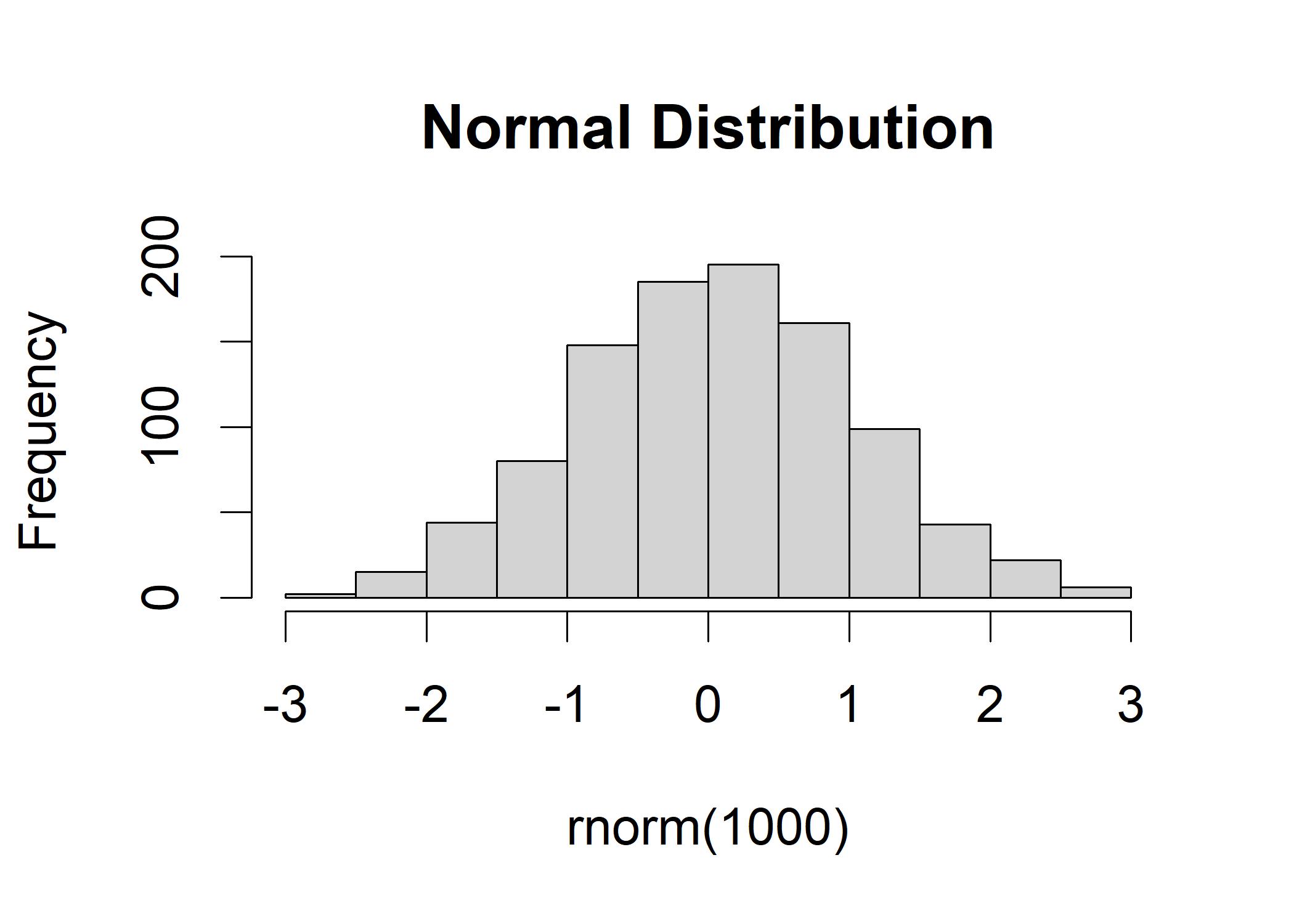
Exponential Distribution has a long tail on the right side.
Lognormal Distribution has a long tail on the left side.
Poisson Distribution has a long tail on the right side.
The Poisson distribution is a discrete probability distribution that expresses the probability of a given number of events occurring in a fixed interval of time and/or space if these events occur with a known constant rate and independently of the time since the last event. It is used to model the number of times an event occurs in an interval. For example, the number of cars passing a certain point on a highway in one hour.
R illustration:
hist(rpois(1000, lambda = 1)) # lambda is the rate parameter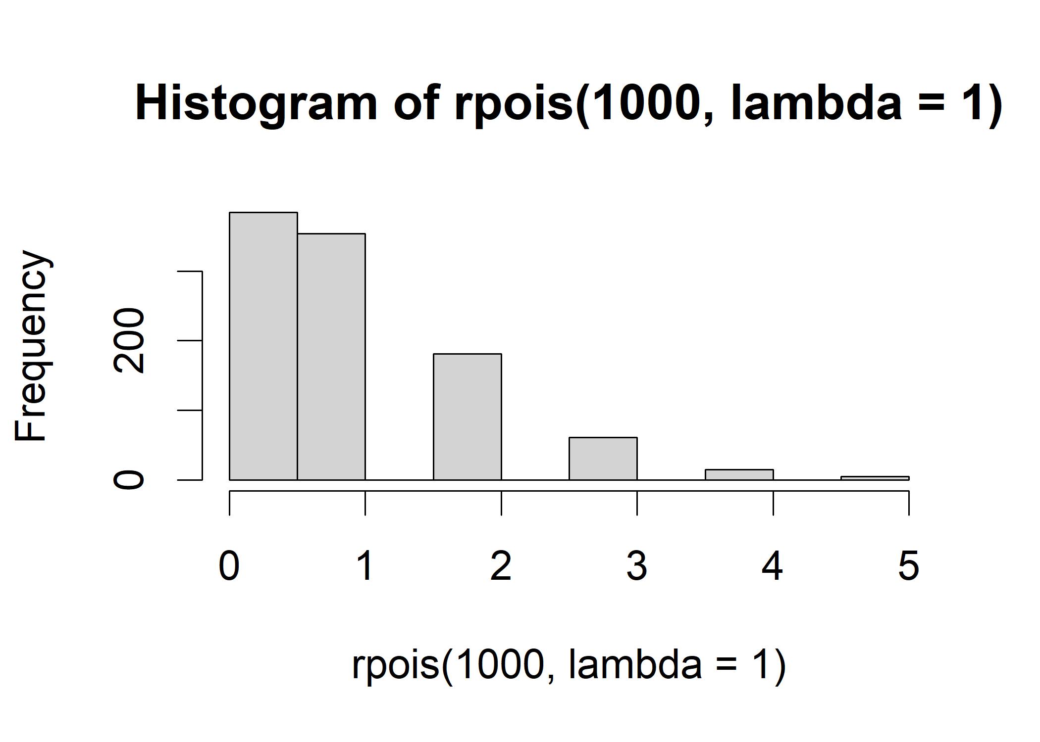
Skewness
- The skewness is a measure of the asymmetry of the probability distribution of a real-valued random variable about its mean. It is useful to show the degree of asymmetry of the distribution. The skewness is positive if the tail on the right side of the distribution is longer or fatter than the tail on the left side. The skewness is negative if the tail on the left side of the distribution is longer or fatter than the tail on the right side. The skewness is zero if the two tails are of the same length.
- r illustration:
# zero_skewness <- rnorm(1000, mean = 100, sd = 10)
# positive_skewness <-rnorm(1000, mean = 100, sd = 10) + 10000
# negative_skewness <- rnorm(1000, mean = 100, sd = 10) - 10000
# skewness(zero_skewness)
# skewness(positive_skewness)
# skewness(negative_skewness)The kurtosis measures the amount in the tails and outliers of the distribution. The kurtosis is positive if the tails are fatter than the normal distribution. The kurtosis is negative if the tails are thinner than the normal distribution. The kurtosis is zero if the tails are the same as the normal distribution.
1.1.4 Moments
The moments are the measures of the central tendency and the dispersion of a distribution. The first moment is the mean/expected value, the second moment is the variance, and the third moment is the skewness. The fourth moment is the kurtosis. The higher moments are the higher-order central moments.