2.2 Probabilities in the Long Run

The probability shown before is built for simple events that are not necessarily representative of a large realm of probability. If a model can represent a phenomenon, we can utilize it to generate long-run outcomes.

2.2.1 Sampling

Sampling is a process of selecting a subset of a population to represent the whole population. Sampling error is the difference between the sample statistic and the population parameter. For instance, the sample mean is an estimate of the population mean.

Random sampling with replacement To ensure the probability of each draw won’t affect the probability of the next draw, random sampling with replacement will put back the original entity.

R illustration Suppose we are throwing a dart landing at an angle between 0 and 180 degrees, every of which the probability is the same. Now we use the runif package to generate 1000 random numbers from the uniform distribution.

dart_angle <- runif(1000, min = 0, max = 180) # generate 1000 random numbers from the uniform distribution
head(dart_angle)
## [1]  81.67627 112.33222  51.05470  16.28059 105.99043 155.01308
hist(dart_angle, breaks = 20, main = "Histogram of dart angle", xlab = "Angle", ylab = "Frequency")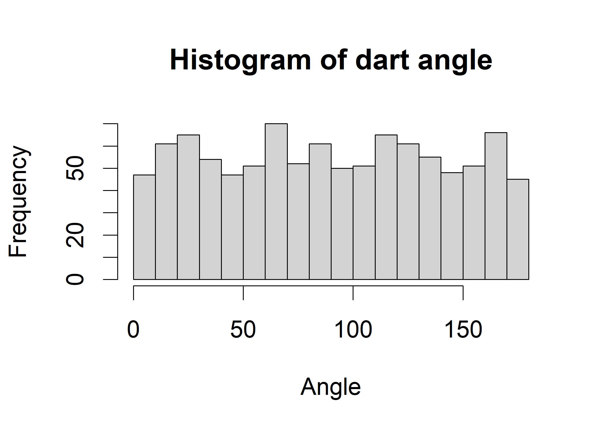

Now we sample 5 elements from dart_angle with replacement.

sample(dart_angle, size = 5, replace = TRUE)
## [1]  73.99757  30.81353  42.78605 133.37863 166.96984

Every time we run this command will get different results because of its randomness and replacement. We pick up the average to represent the sample.

mean(sample(dart_angle, size = 5, replace = TRUE))
## [1] 91.0178

It is limited to see infer the parameter of the population by just a few samples. To see what will happen across different samples over the long course, we replicate the process using replicate() function in R. The first parameter is the replication time and the second parameter is the process we want to replicate.

replicate(4, mean(sample(dart_angle, size = 5, replace = TRUE)))
## [1] 106.4498 112.8199 128.4687 127.5649

Let’s now make it larger and plot the histogram of the distribution of samp_dis. As shown in the following figure, we can see that the distribution looks like a normal distribution where most elements center around the mean.

samp_dis <- replicate(1000, mean(sample(dart_angle, size = 5, replace = TRUE)))
hist(samp_dis)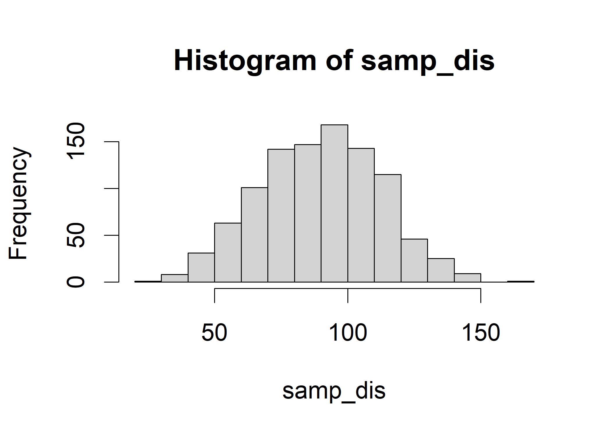

If we further inspect the mean of the original data dart_angle and the grand mean of the mean of each sample groups, we can see that these two means are similar, indicating that when we sample for a long run, the mean of the sample distribution matches the mean of the original data. You hardly ever obtain a sample that exactly mirrors the population. However, it is also uncommon to find a sample whose mean is significantly different from or similar to the population mean.

mean(dart_angle) # mean of the original data
## [1] 89.44857
mean(samp_dis) # grand mean of the mean of each sample groups
## [1] 89.78681