5.3 The Bayesian Approach to ANOVA and R Illustration
The previous approach do not tell us the probability of the support or against the null hypothesis. The Bayesian approach to ANOVA is to use the posterior probability of the group means to assess whether the group means differ.
##
  |
  |                                                                                                                                               |   0%
  |
  |===============================================================================================================================================| 100%
##
## Iterations = 1:10000
## Thinning interval = 1
## Number of chains = 1
## Sample size per chain = 10000
##
## 1. Empirical mean and standard deviation for each variable,
##    plus standard error of the mean:
##
##                 Mean     SD Naive SE Time-series SE
## mu           33.0797  1.719  0.01719        0.01744
## precipGrp-1   2.3875  2.192  0.02192        0.02307
## precipGrp-2  -1.9405  2.145  0.02145        0.02255
## precipGrp-3  -0.4470  2.111  0.02111        0.02149
## sig2        179.0792 33.725  0.33725        0.35638
## g_precipGrp   0.3617  1.355  0.01355        0.01367
##
## 2. Quantiles for each variable:
##
##                  2.5%       25%      50%      75%   97.5%
## mu           29.71151  31.93786  33.0711  34.2267  36.419
## precipGrp-1  -1.72218   0.89449   2.3370   3.8247   6.853
## precipGrp-2  -6.36481  -3.32917  -1.8863  -0.4860   2.130
## precipGrp-3  -4.67414  -1.82586  -0.4360   0.9375   3.687
## sig2        124.83979 155.10633 174.8958 198.4794 256.045
## g_precipGrp   0.03511   0.08729   0.1576   0.3246   1.787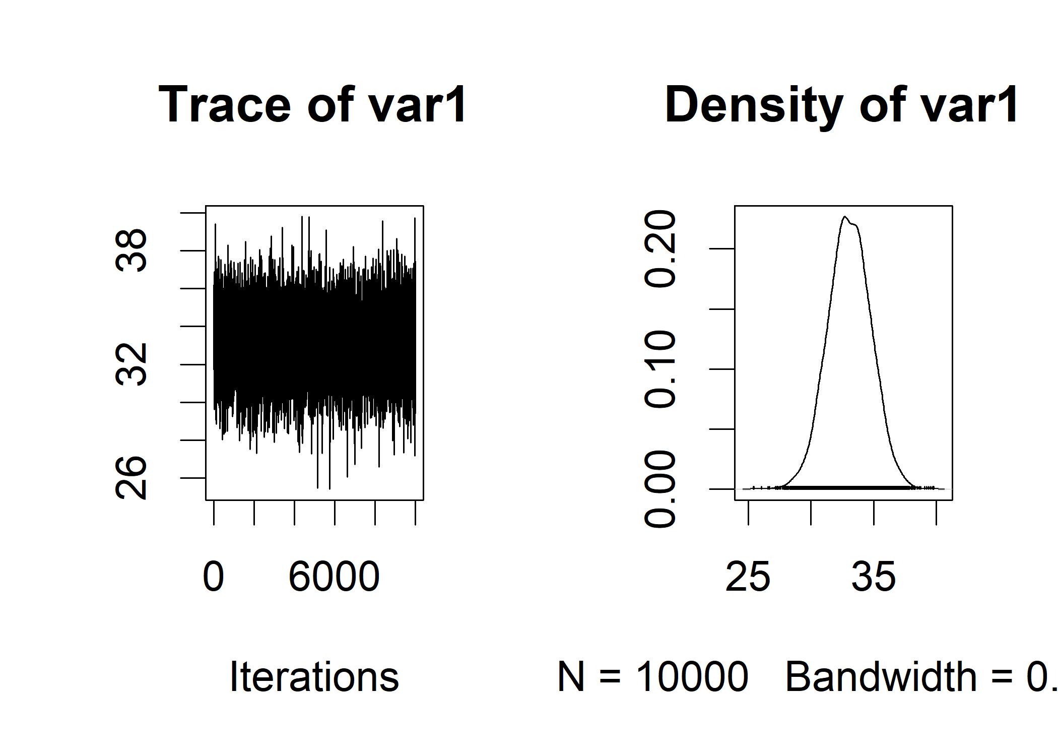
The mcmcOut tell us two sections of information.
- Empirical mean and standard deviation
- These mean values represent the posterior distribution of each population parameter over the 10,000 samples that posterior() generated using MCMC. sig2: the population variance. The “naive” standard error, or Naive SE, is calculated by dividing the standard deviation by the square root of 10,000. Compared to the MCMC run, the Time Series SE is calculated slightly differently.
- Quantiles for each variable
- Any pair of the groups must have distinct HDIs in order for them to be plausibly different from one another. Each of the 95% HDIs crosses 0. As a result, it can be concluded that all three of the groups were selected from the same population because none of the group means can be reasonably said to depart from the overall mean.
Interpretation of Bayes Factor
precipBayesOut
## Bayes factor analysis
## --------------
## [1] precipGrp : 0.2800937 ±0.01%
##
## Against denominator:
##   Intercept only
## ---
## Bayes factor type: BFlinearModel, JZS
The value of precipGrp represents the odds ratio (research hypothesis / null hypothesis) that supports the research hypothesis.
- Every Bayes factor depicts a contrast between two statistical models, such as the null hypothesis and an alternative hypothesis.
- Instead of merely comparing alternative hypotheses to the null hypothesis, Bayes factors allow for such comparisons.
- Any odds ratio smaller than 3:1 is not significant, odds ratios from 3:1 to 20:1 support the preferred hypothesis, odds ratios between 20:1 and 150:1, and odds ratios higher than 150:1 provide extremely strong support.