6.1 Covariance

One of the most familiar measures of association is the Pearson product-moment correlation (PPMC). It is build upon a concept called covariance. Covariance is a measure of the joint variability of two random variables. It is the directional relationship between the returns on two assets. Imaging if we sample a variety of fire and measure the amount of fuel and the heat of each fire, we can partition the variance of the heat and fuel variables into the shared part by both of them and the independent part that infused by each variable. The shared part is called covariance. Formally, the covariance between two variables \(X\) and \(Y\) is defined as: \[cov(X,Y) = E[(X-E[X])(Y-E[Y])]\] where \(E[X]\) and \(E[Y]\) are the expected values of \(X\) and \(Y\) respectively. Correlation coefficients, which depend on the covariance, are a dimensionless measure of linear dependence.

6.1.1 R illustration

We first generate random samples where no association exists between the variables. We generate two samples of data following normal distribution with the mean and standard deviation of 0 and 1, respectively.

set.seed(10)
wood <- rnorm(24)
heat <- rnorm(24)
mean(wood)
## [1] -0.2827574
mean(heat)
## [1] -0.427342
sd(wood)
## [1] 0.9415208
sd(heat)
## [1] 0.8083186
plot(wood, heat)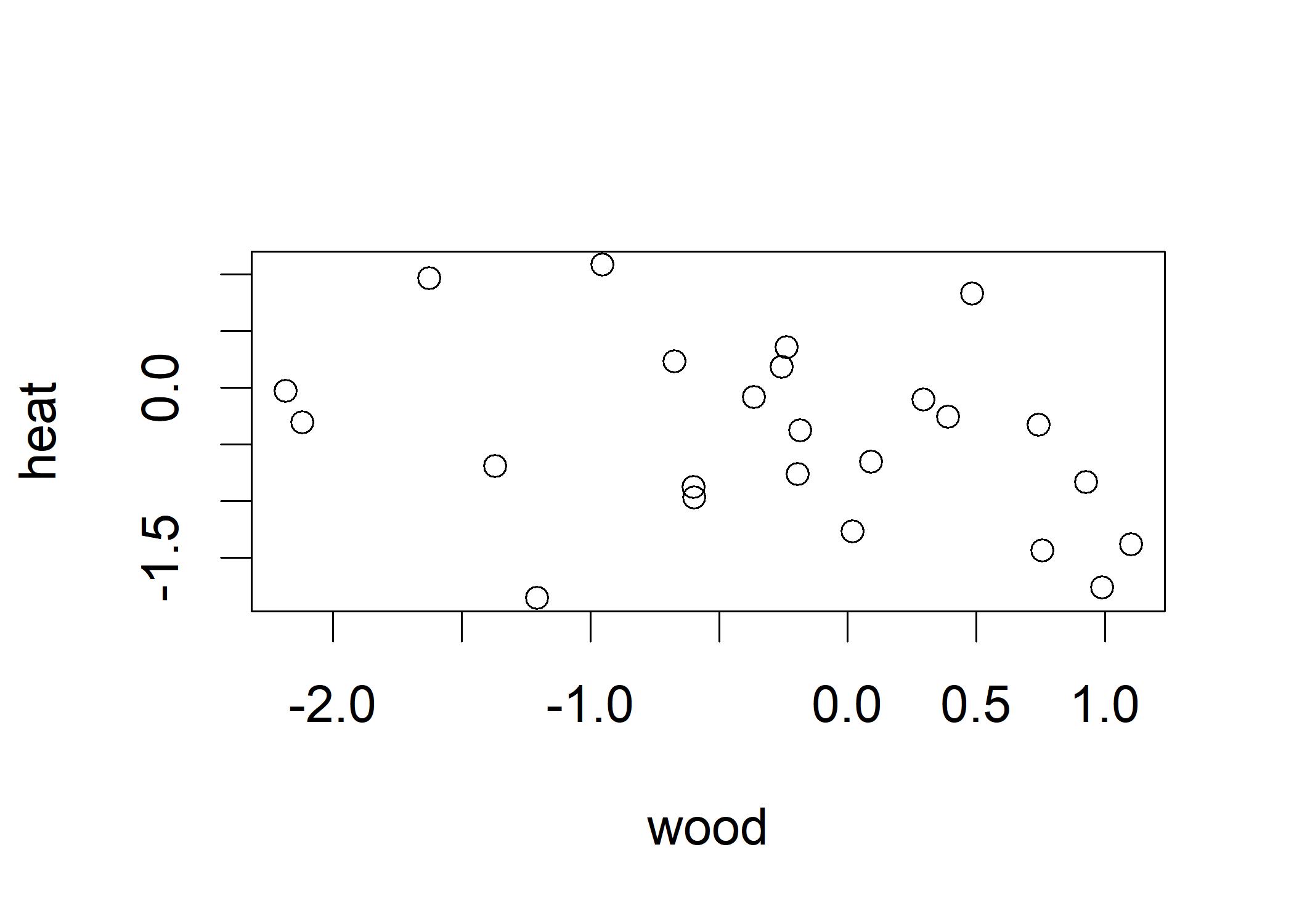

This plot shows that the points situated around the respective mean of each variable. These two variables follow the standard normal distribution where most points are around the range of two standard deviation away from the mean. These two variables can be called as standard normal variables, meaning that each observation of wood and heat is a z-score (the number of standard deviations is above the mean). We can get a sense how much two variables covary by calculating the products of their respective z-scores. Thinking of each observation has two dimensions, we can calculate the covariance by multiplying the z-scores of each dimension. If the z-scores are both positive or both negative, the covariance is positive. If one z-score is positive and the other is negative, the covariance is negative. For instance, we create the cross-product of the z-scores of wood and heat.

cpWH <- wood * heat # cross-product of wood and heat
mean(cpWH)
## [1] -0.1180109
hist(cpWH)

In this figure, we observe more than a half of the cross-products are near 0 and the mean of cross-product between pairs of variables is also near 0, indicating that no association exists between the variables.

Next, we generate samples with positive association between the variables.

# mix the two old variables by taking half of its influence from the wood variable
# and half of its influence from the existing heat variable
newHeat <- wood/1.41 + heat/1.41
newHeat
##  [1] -0.88400840 -0.39568376 -1.46020282 -1.04349400  0.13672633  0.09646367 -2.17150116 -0.31320715 -0.46674209 -0.05074641 -0.19727949 -0.48208004
## [13]  0.08783948 -0.54726387  0.29563555 -0.39873455  0.09333868 -0.67921650  0.06869413  0.93436342 -1.10919335 -1.57028523 -0.31371687 -1.71650346
mean(newHeat)
## [1] -0.5036166
sd(newHeat)
## [1] 0.7237453

The newHeat now have covariance with wood because we inject the variance of wood into the newHeat variable.

cpWnewH <- wood * newHeat
hist(cpWnewH)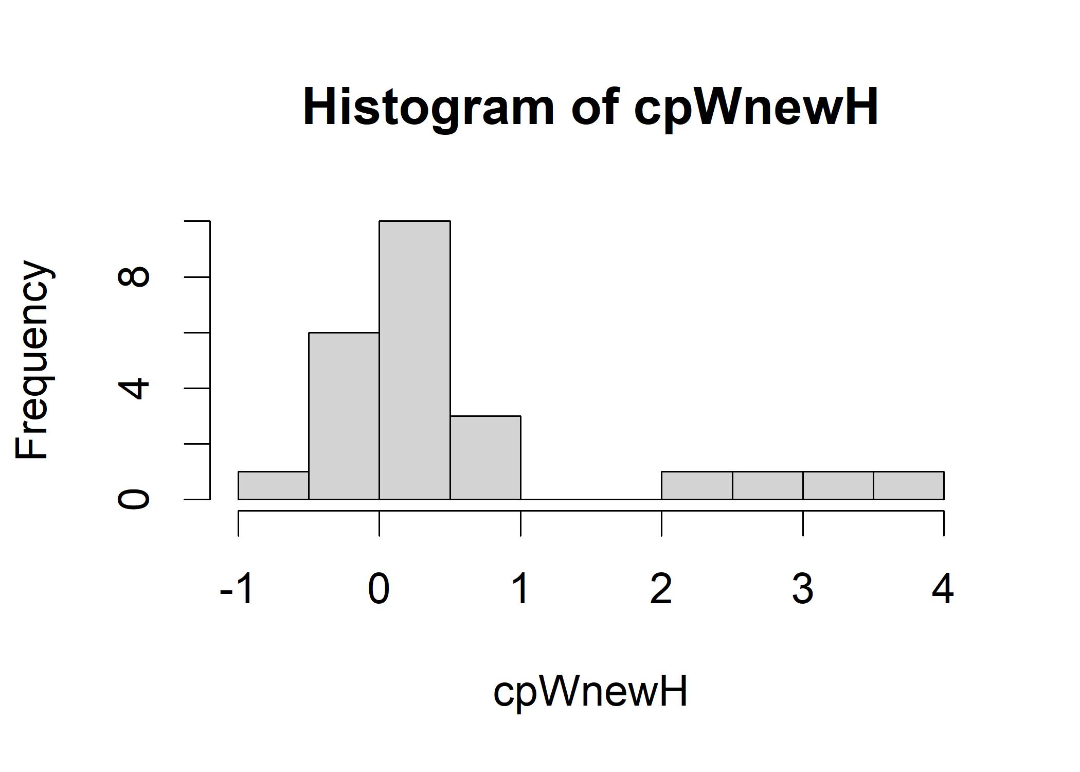

mean(cpWnewH)
## [1] 0.5755081
cor(wood, newHeat)
## [1] 0.6632277

The histogram shows that the cross-product of wood and newHeat is not centered around 0. The mean of the cross-product is also not 0. The mean of the cross-product is 0.57. The cross-product only works if the two variables are both z-scores. The association between wood and newHeat is the mean of the products of the z-scores of wood and newHeat. Formula for Pearson product-moment correlation (PPMC): \[\rho_{X,Y} = \frac{\sum_{i=1}^{n}(x_i - \bar{x})(y_i - \bar{y})}{\sqrt{\sum_{i=1}^{n}(x_i - \bar{x})^2}\sqrt{\sum_{i=1}^{n}(y_i - \bar{y})^2}}\] where \(\rho_{X,Y}\) is the PPMC between variables \(X\) and \(Y\). You may also find “r” in the software, which represents the sample value of the correlation, while \(\rho\) (rho) represents the population value of the correlation.

6.1.2 Inferential Reasoning About Correlation

As mentioned above, the r does not equal to \(\rho\). How much the r differs from \(\rho\) depends on the sample size. The larger the sample size, the closer the r is to \(\rho\). Let’s infer the population correlation between wood and newHeat from the sample correlation by looking at the possible outcomes.

set.seed(12345)
wood <- rnorm(2400)
heat <- rnorm(2400)
fireDF <- data.frame(wood, heat)
samp <- fireDF[sample(nrow(fireDF), 24), ] # sample 24 rows from the data frame
cor(samp)
##             wood        heat
## wood  1.00000000 -0.09362733
## heat -0.09362733  1.00000000

We now replicate the r value of the sample:

corDist <- replicate(5000,cor(fireDF[sample(nrow(fireDF), 24), ])[1,2])
hist(corDist)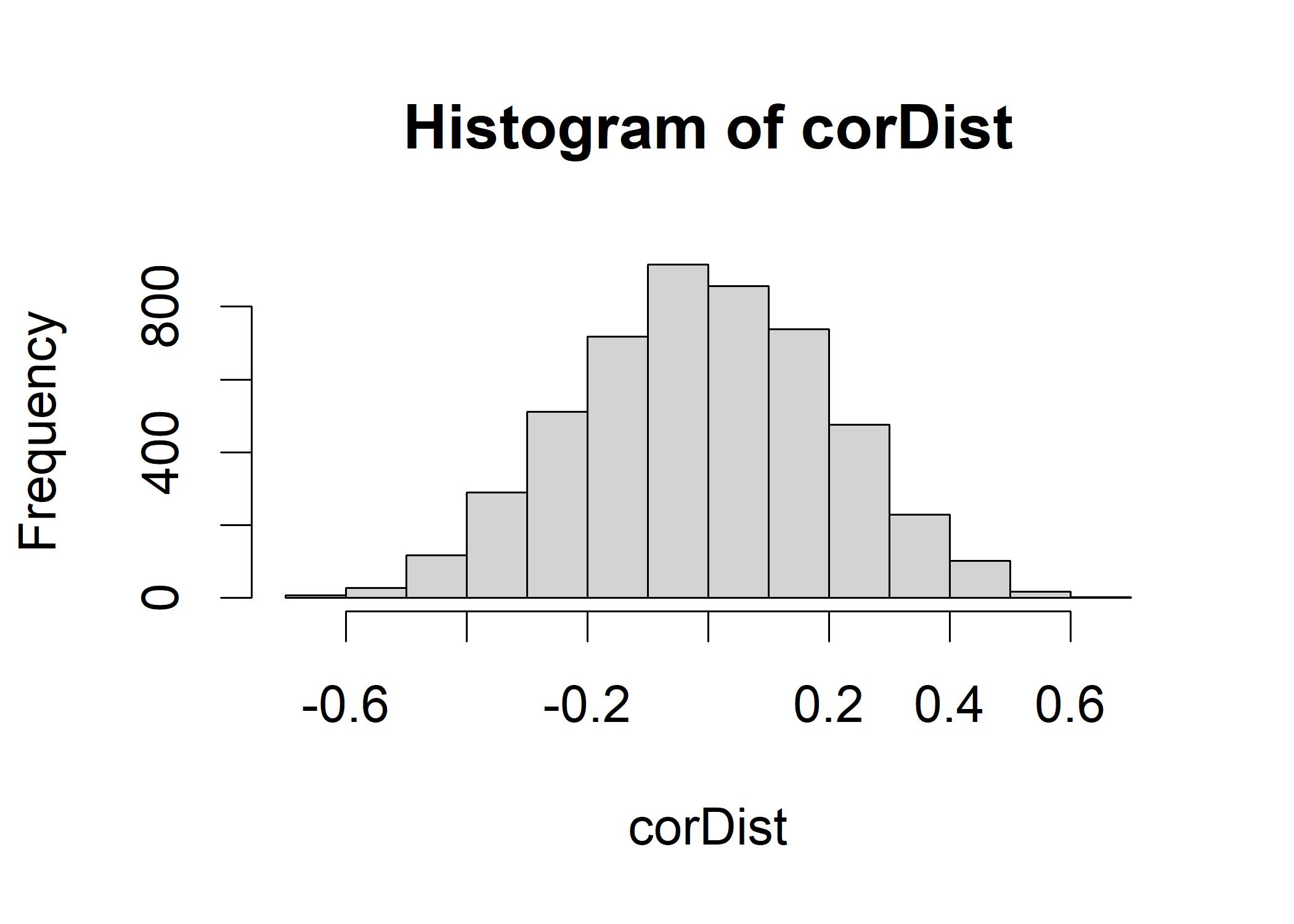

mean(corDist)
## [1] -0.008456108

The \(\rho\) is very close to the center of the empirical sampling distribution we constructed. If you square the r value, you will get the proportion of the variance of one variable that is shared with the other variable (R-squared).