3.1 Confidence Intervals

A confidence interval is a range of values that we are confident contains the true value of the population parameter. Let’s use a dataset called “mtcars” that contains a sample of 32 vehicles with attributes such as mileage and gross horsepower to showcase an inferential statistical analysis. Research question: Do cars with automatic transmissions get larger or smaller gross horsepower than cars with manual transmissions?

Here we show the mean of the gross horsepower for cars with automatic and manual transmissions.

mean(mtcars$hp[mtcars$am == 0]) # automatic transmission
## [1] 160.2632
mean(mtcars$hp[mtcars$am == 1]) # manual transmission
## [1] 126.8462

It seems like we can conclude that cars with automatic transmissions get larger gross horsepower than cars with manual transmissions based on the sample means. However, the sample means is just a point estimate of the original population, and we are not sure how good the estimate is. This uncertainty can be bounded by applying inferential statistics.

In comparison to a sample with low variability, a sample with high variability reduces our confidence in the underlying population mean. We draw the boxplot to compare distributions and variability where the x-axis is the independent variable am and y is the dependent variable hp. To explain the boxplot, the lower boundary of the box represents the first quartile and the upper boundary of the box represents the third quartile. The solid line in the middle of the box represents the median. The circle represents the outliers. You can see that in the case of manual transmissions, the median is quite close to the first quartile, suggesting that 25% of the cases are clustering in the small region between about 110 to 115.

The boxplot shows a sense that these two groups are different. The boxes do not overlap, the different in the heights suggests that their standard deviation differs. Despite the observations, we cannot be certain because it could be that the samples are different. Let’s try to replicate it using the idea from the last chapter.

boxplot(hp ~ am, data = mtcars)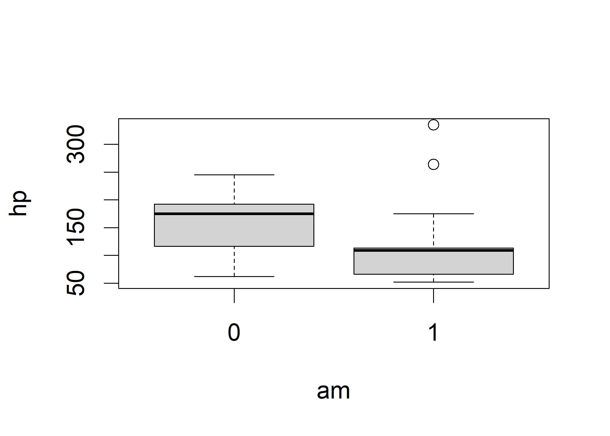

We explore the variability of sample means with repitition sampling. First, we draw a sample of n=19 from the automatic transmission group and n=13 from the manual transmission group. We calculate their mean difference.

at_mean <- mean(sample(mtcars$hp[mtcars$am == 0], 19, replace = TRUE))
mn_mean <- mean(sample(mtcars$hp[mtcars$am == 1], 13, replace = TRUE))
at_mean - mn_mean
## [1] 13.86235

Let’s replicate it by 100 times and plot the histogram of the distribution. The figure suggests that most cases differ by around 25. We might interpret it as “There may be a difference in horsepower between manual and automatic transmissions of roughly 25, but in rare occasions, that gap could be as little as -30 or as much as 80.”. The width of the span from -20 to 80 signifies the different possibilities.

meanDiffs <- replicate(100, mean(sample(mtcars$hp[mtcars$am == 0], 19, replace = TRUE)) - mean(sample(mtcars$hp[mtcars$am == 1], 13, replace = TRUE)))
hist(meanDiff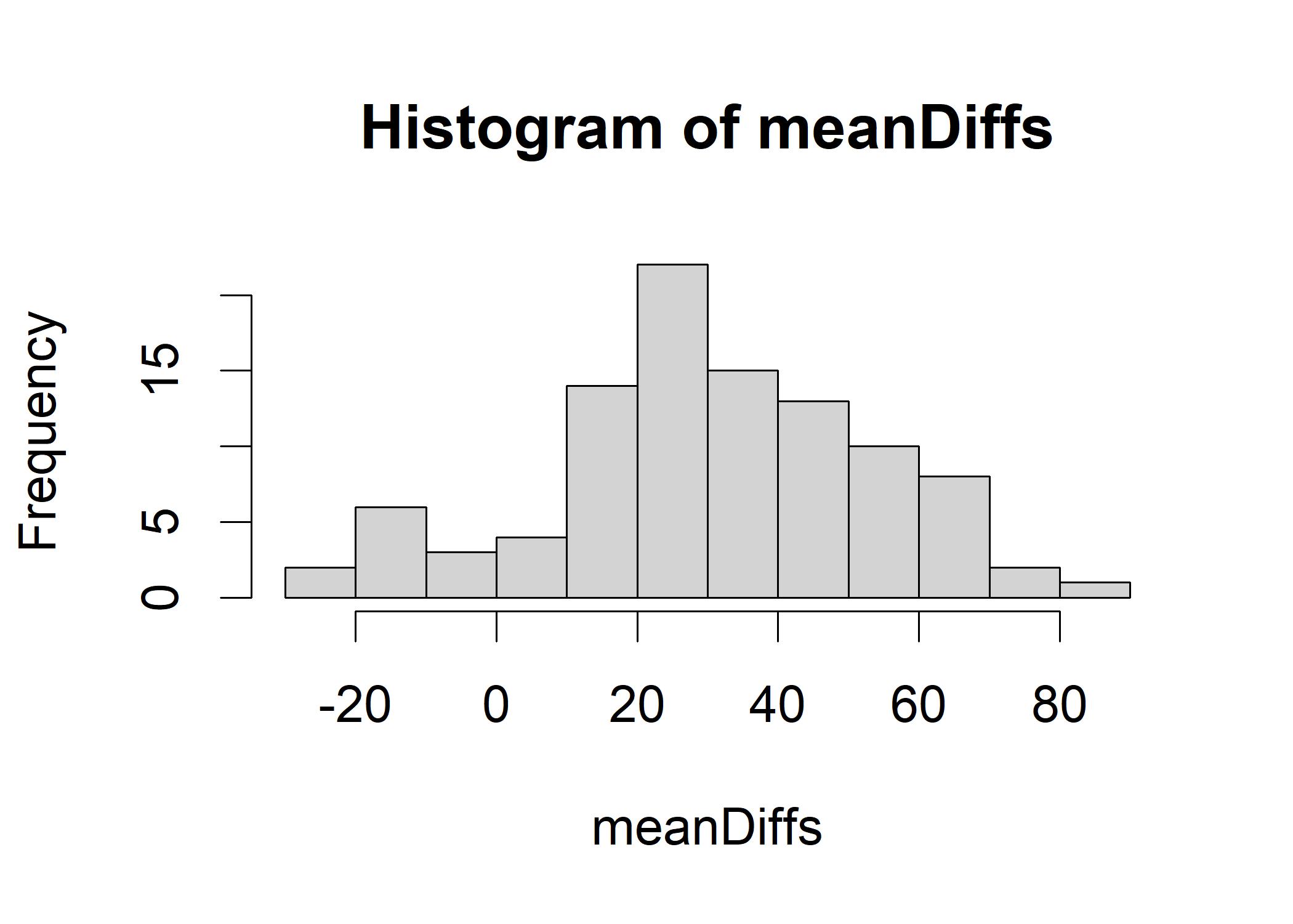s)

For a more decent analysis as follows, we can say that with a difference of roughly 25, automatic transmissions may offer higher horsepower than manual transmissions, but for 95% of the simulated mean differences, that difference might be as high as 69.26478 or as low as -19.16630. As a measure of our uncertainty, the width of this range—about plus or minus 25 — shows what may occur in around 95 out of every 100 trials if we repeatedly gathered horsepower data for vehicles with the two different types of transmissions.

quantile(meanDiffs, c(0.025, 0.975))
##      2.5%     97.5% 
## -19.16630  69.26478

3.1.1 Confidence Interval of T-test

Now let’s conduct Student’s t-test using the following command. The t-test is to generalize to a population of mean differences using sample data from two independent groups of observations. The t-test procedure used these two samples to calculate a confidence interval.

t.test(hp ~ am, data = mtcars)
## 
##  Welch Two Sample t-test
## 
## data:  hp by am
## t = 1.2662, df = 18.715, p-value = 0.221
## alternative hypothesis: true difference in means between group 0 and group 1 is not equal to 0
## 95 percent confidence interval:
##  -21.87858  88.71259
## sample estimates:
## mean in group 0 mean in group 1 
##        160.2632        126.8462

It is worth noting that the confidence interval from our t-test above does not necessarily include the actual population value of the mean difference. The 95% represents a long-term prediction of what would occur if the study were reproduced, with new samples taken from the populations each time, and new confidence intervals calculated. The animation samples from the normal distribution produce 50 distinct confidence intervals surrounding a population mean of 0. Each confidence interval looks like “I” and the circle in the “I” represents the mean of each sample. The red “I” means that the confidence interval does not overlap with the population mean. 96% of the sample mean overlaps with the population mean. So the confidence interval means the proportion of constructing confidence intervals that would likely contain the true population mean. And since we typically only have the opportunity to conduct one study and collect one sample, we will never be able to determine if our specific confidence interval falls within the 95th or the 5th percentile. A 95% confidence interval means that we would be likely to discover that whatever confidence interval we generated in a given study did contain the actual population value in 95 out of 100 study replications. This is not a statement about the exact confidence interval we constructed using this particular data set; rather, it is a statement about probabilities over the long term. The true population value may or may not be contained within this specific confidence interval.

# install.packages("animation")
library(animation)
conf.int(level = 0.95, size = 100)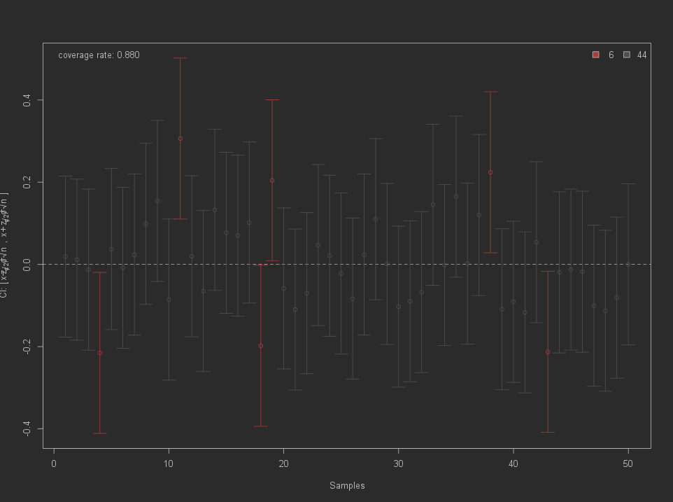

image