8.2 Bayesian Approach of Interaction in ANOVA

Let’s look at the Bayesian evidence for the interaction effect.

library(BayesFactor)
aovOut3 <- anovaBF(weightgain ~ source*type, data=weightgain)
## 
  |                                                                                                                                                     
  |                                                                                                                                               |   0%
  |                                                                                                                                                     
  |====================================                                                                                                           |  25%
  |                                                                                                                                                     
  |========================================================================                                                                       |  50%
  |                                                                                                                                                     
  |===========================================================================================================                                    |  75%
  |                                                                                                                                                     
  |===============================================================================================================================================| 100%
aovOut3
## Bayes factor analysis
## --------------
## [1] source                      : 0.4275483 ±0.01%
## [2] type                        : 2.442128  ±0.01%
## [3] source + type               : 1.079618  ±0.75%
## [4] source + type + source:type : 1.713419  ±0.89%
## 
## Against denominator:
##   Intercept only 
## ---
## Bayes factor type: BFlinearModel, JZS

We only found weak evidence (1/0.428=2.34) in favor of the null hypothesis of no effect for source. We also found weak evidence in favor of the alternative hypothesis of effect for type and interaction. We can use the fraction of the model [3] and [4] to explore whether the model that includes the interaction is noticebly better than the main effects-only model.

aovOut3[4]/aovOut3[3] # What’s the odds ratio of model 4 vs. model 3?
## Bayes factor analysis
## --------------
## [1] source + type + source:type : 1.587061 ±1.16%
## 
## Against denominator:
##   weightgain ~ source + type 
## ---
## Bayes factor type: BFlinearModel, JZS

The results suggest that we in favor of the model that includes the interaction term.

We examine the posterior distribution of parameters for the interaction effect.

mcmcOut <- posterior(aovOut3[4],iterations=10000) # Run mcmc iterations
boxplot(as.matrix(mcmcOut[,2:5]), main="posterior distributions for deviations from mu (the grand mean) for the source main effect and the type main effect")

boxplot(as.matrix(mcmcOut[,6:7]), main="posterior distributions for deviations from mu (the grand mean) for one of the interaction contrasts. Beef&High versus Beef&Low")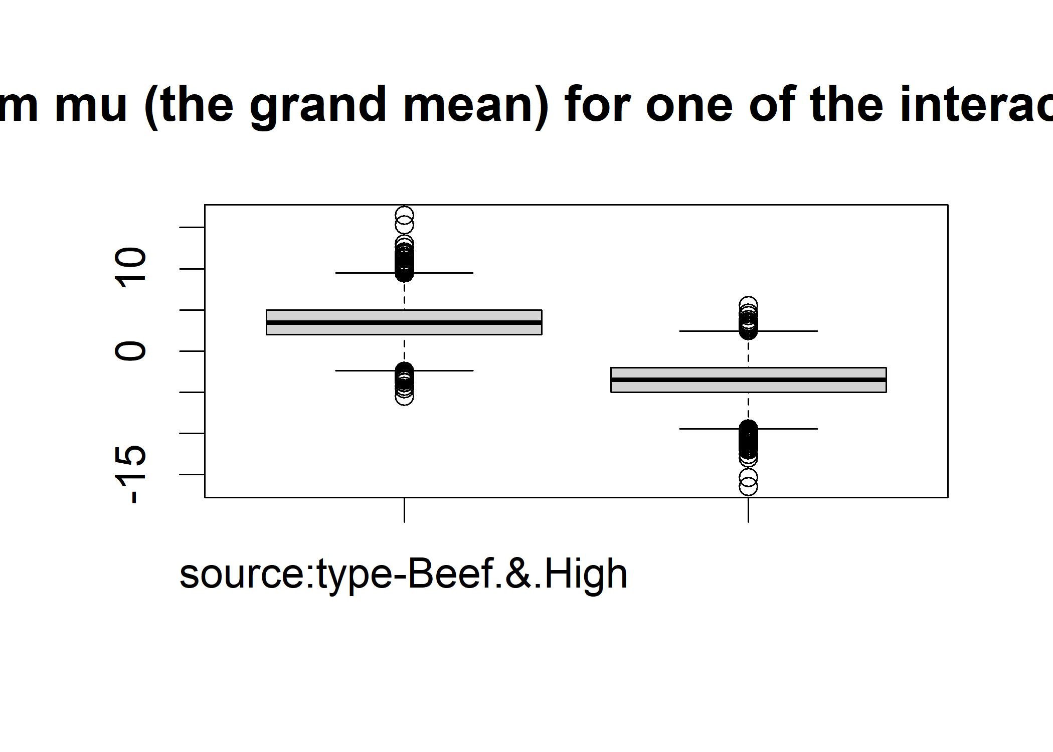

The first plot displays the main effects and the second plot displays the interaction effect. In the first plot, compare the two left pair of boxes which overlap substantially suggesting that the source has no credible difference in weight gain. The right pair of boxes overlap to some degree and confirmed wha tthe weak Bayes factor shows: the main effect of type is weak. In the second plot, the two boxes are far apart suggesting that the interaction effect is significant.

We can use plotmean() to make a means plot that shows confidence intervals.

# install.packages("gplots")
library("gplots")
plotmeans(weightgain ~ interaction(source,type,sep =" "), data = weightgain, connect = list(c(1,2),c(3,4)))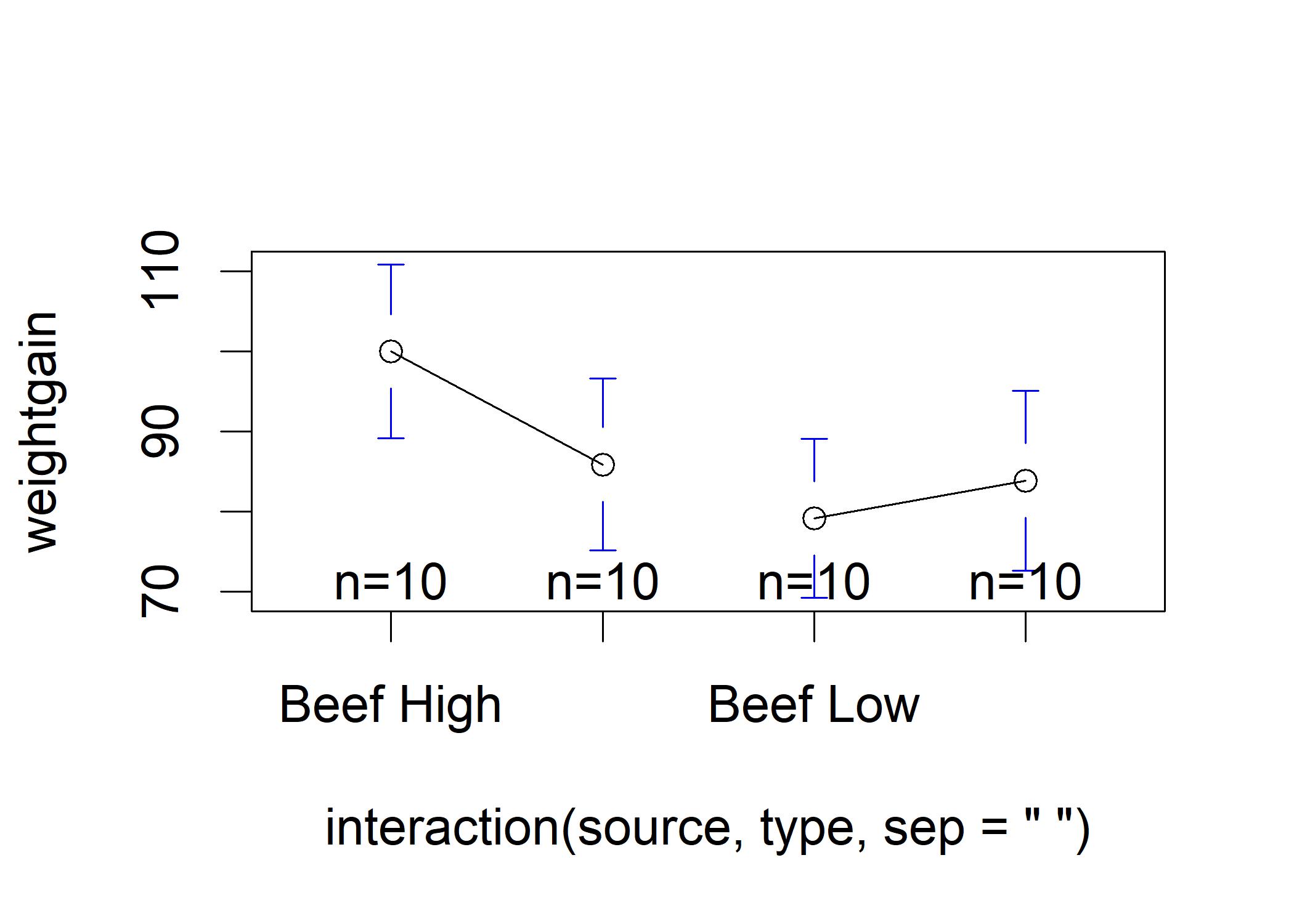

The figure suggests that the differences in the groups is not large enough to overcome the uncertainty due to sampling error. The eta-squared effect size for the main effect of type is 1300/(221 + 1300 + 884 + 8049) = 0.12, which means the type of feed (high protein vs. low protein) accounts for 12% of the variability in weight gain.

Standard Error Standard error is the standard deviation of the sampling distribution of a statistic. It is a measure of the accuracy with which a sample statistic represents a population parameter. The formula for standard error is: \[SE = \frac{\sigma}{\sqrt{n}}\] where \(\sigma\) is the standard deviation of the population and \(n\) is the sample size. The standard error represents the variability in our sampling distribution, then plus or minus two standard errors covers the whole central 95% region of the sampling distribution.