9.1 Bayesian Estimation of Logistic Regression

The goal of the Bayesian analysis is to use a set of weakly informative prior distributions to estimate the posterior distribution of the parameters. The outcomes include posterior distributions for each coefficient, where the mean value serves as our point estimate of the coefficient and the distribution around the mean identifies the greatest density region where the population value of the coefficient is most likely to fall. Now we use “Chilean citizens”, two metric variables, age and income to predict whether individual vot “Y” or “N”.

# install.packages("Chile")
library(car)
ChileY <- Chile[Chile$vote == "Y",]
ChileN <- Chile[Chile$vote == "N",]
ChileYN <- rbind(ChileY,ChileN)   # Make a new dataset with those
ChileYN <- ChileYN[complete.cases(ChileYN),]  # Get rid of missing data
ChileYN$vote <- factor(ChileYN$vote,levels=c("N","Y")) # Simplify the factor
boxplot(age ~ vote, data=ChileYN)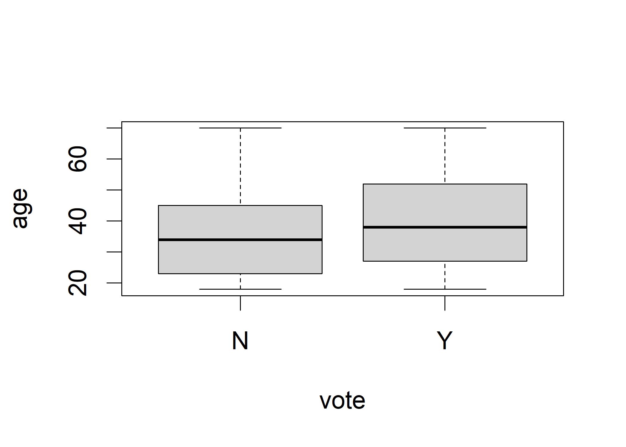

# install.packages("MCMCpack")
library(MCMCpack)
ChileYN$vote <- as.numeric(ChileYN$vote) - 1 # Adjust the outcome variable
bayesLogitOut <- MCMClogit(formula = vote ~ age + income, data = ChileYN)

summary(bayesLogitOut)
## 
## Iterations = 1001:11000
## Thinning interval = 1 
## Number of chains = 1 
## Sample size per chain = 10000 
## 
## 1. Empirical mean and standard deviation for each variable,
##    plus standard error of the mean:
## 
##                   Mean        SD  Naive SE Time-series SE
## (Intercept) -7.602e-01 1.452e-01 1.452e-03      4.849e-03
## age          1.935e-02 3.317e-03 3.317e-05      1.089e-04
## income      -3.333e-07 1.151e-06 1.151e-08      3.723e-08
## 
## 2. Quantiles for each variable:
## 
##                   2.5%        25%        50%        75%      97.5%
## (Intercept) -1.044e+00 -8.588e-01 -7.609e-01 -6.639e-01 -4.710e-01
## age          1.278e-02  1.711e-02  1.930e-02  2.157e-02  2.584e-02
## income      -2.549e-06 -1.113e-06 -3.662e-07  4.437e-07  1.926e-06

The output shows the posterior distribution of the intercept and the coefficients on age and income, calibrated as log-odds. The mean column show the point estimate for the intercept and the coefficient. The SD column shows the standard error in the output from the traditional logistic regression. The second section shows the 95% HDI for the intercept and the coefficient.

plot(bayesLogitOut[,1], main="Posterior Distributions of the Intercept and Coefficients")

The left plot shows the trace of the progress of MCMC analysis. The right plots display each coefficient’s most likely place graphically. In any distribution, the true population value of each coefficient is more likely to be someplace near the center than it is to be far out in the tails. Now, we examine the posterior distribution of age in terms of regular odds.

ageLogOdds <- as.matrix(bayesLogitOut[,"age"])  # Create a matrix for apply()
ageOdds <- apply(ageLogOdds,1,exp)  # apply() runs exp() for each one
hist(ageOdds)           # Show a histogram
abline(v=quantile(ageOdds,c(0.025)),col="black") # Left edge of 95% HDI
abline(v=quantile(ageOdds,c(0.975)),col="black") # Right edge of 95% HDI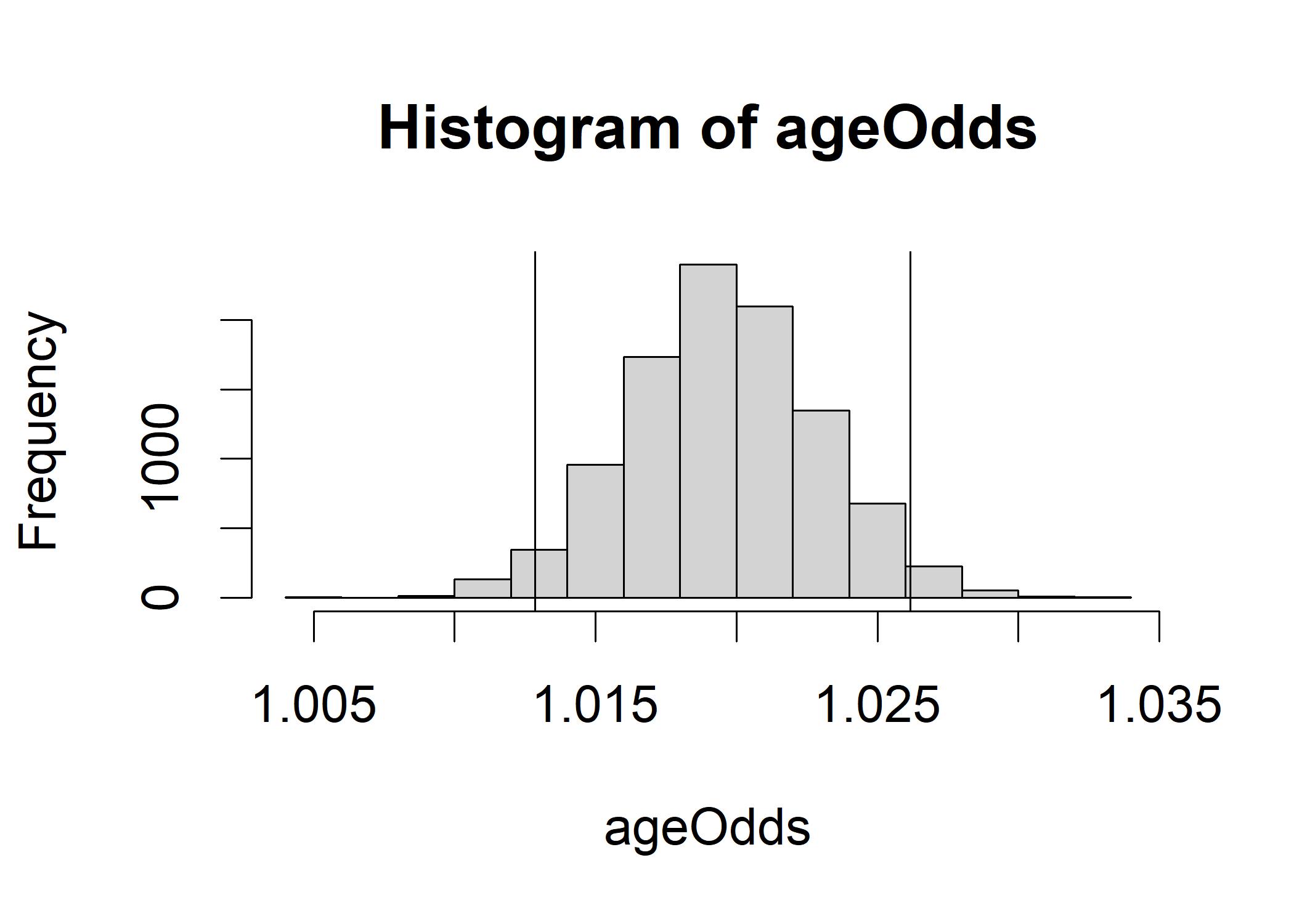

The histogram shows a symmetric distribution center on about 1.02. An increase of about 2% in the likelihood of a Yes vote for an increase in age of 1 year. The95% HDI ranges from 1.013 to 1.026.