10.3 Finding Change Points in Time Series

Change-point analysis is used to examine whether an intervention or natural event has caused a change in the behavior of a time series. Let’s look at European stock market data:

str(EuStockMarkets)
##  Time-Series [1:1860, 1:4] from 1991 to 1999: 1629 1614 1607 1621 1618 ...
##  - attr(*, "dimnames")=List of 2
##   ..$ : NULL
##   ..$ : chr [1:4] "DAX" "SMI" "CAC" "FTSE"
plot(EuStockMarkets)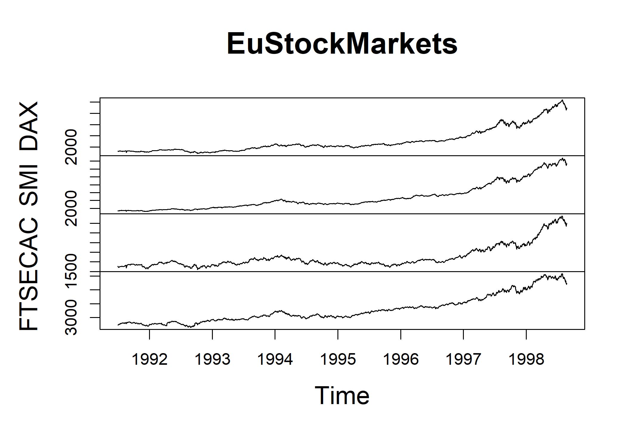

We want to find out the particular inflection point when the average value of stocks increase substantially.

# install.packages("changepoint")
library(changepoint)
DAX <- EuStockMarkets[,"DAX"]
DAXcp <- cpt.mean(DAX)
DAXcp
## Class 'cpt' : Changepoint Object
##        ~~   : S4 class containing 12 slots with names
##               cpttype date version data.set method test.stat pen.type pen.value minseglen cpts ncpts.max param.est 
## 
## Created on  : Thu Nov 10 04:05:49 2022 
## 
## summary(.)  :
## ----------
## Created Using changepoint version 2.2.4 
## Changepoint type      : Change in mean 
## Method of analysis    : AMOC 
## Test Statistic  : Normal 
## Type of penalty       : MBIC with value, 22.585 
## Minimum Segment Length : 1 
## Maximum no. of cpts   : 1 
## Changepoint Locations : 1467

The method of analysis is AMOC (at most one change). The “Type of Penalty” in the output refers to a mathematical formulation that determines how sensitive the algorithm is to detecting changes. Bigger penalty means only indentify the very largest shifts in the time series. The default for AMOC is Modified Bayesian Information Criterion (MBIC). We use the following plot to visualize where the change occur and how big the shift is:

plot(DAXcp,cpt.col="grey",cpt.width=5)

The DAX stock index is sluggishly hovering around 2,000 before the first quarter of 1997. The index unexpectedly increases to a higher level, just over 4,000, after the first quarter of 1997. The mean level of the index during the entire time period represented by each horizontal grey line. Using change-point analysis, we could detect shifts in the mean of the time series as the intervention is added and removed.

Instead of mean, cpt.var() is used to detect changes in the variability of a time series over time.

cpt.var(diff(EuStockMarkets[,"DAX"]))
## Class 'cpt' : Changepoint Object
##        ~~   : S4 class containing 12 slots with names
##               cpttype date version data.set method test.stat pen.type pen.value minseglen cpts ncpts.max param.est 
## 
## Created on  : Thu Nov 10 04:05:49 2022 
## 
## summary(.)  :
## ----------
## Created Using changepoint version 2.2.4 
## Changepoint type      : Change in variance 
## Method of analysis    : AMOC 
## Test Statistic  : Normal 
## Type of penalty       : MBIC with value, 22.58338 
## Minimum Segment Length : 2 
## Maximum no. of cpts   : 1 
## Changepoint Locations : 1480

This result indicates that the variability of the DAX stock index has increased substantially in 1997.