8.3 Interation in Regression
We use “environmental” dataset contains two variables: ozone and radiation, and there is interaction between the two variables. However, the interaction effect is affected by the wind speed.
# install.packages("lattice")
library(lattice)
data(environmental)
plot(environmental$radiation,environmental$ozone)
# This grey line shows what happens when we only consider # the data with wind
# speeds above the median wind speed
hiWind <- subset(environmental, wind > median(environmental$wind))
hiLmOut <- lm(ozone ~ radiation,data=hiWind)
abline(hiLmOut,col="grey")
# This dotted black line shows what happens when we only consider
# the data with wind speeds at or below the median wind speed
loWind <- subset(environmental, wind <= median(environmental$wind))
loLmOut <- lm(ozone ~ radiation,data=loWind)
abline(loLmOut,col="black",lty=3)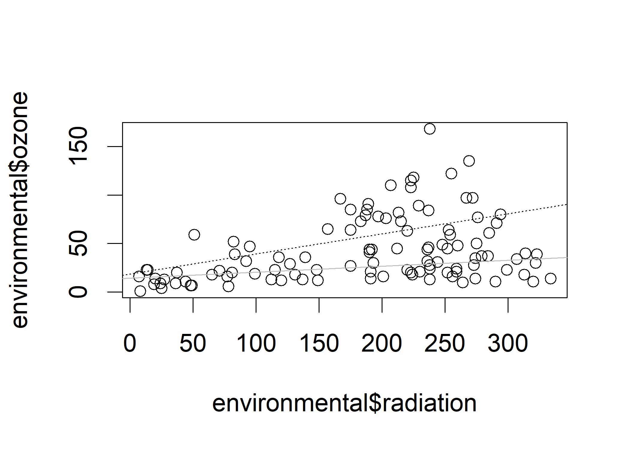 In this figure, the slope of the dotted line (low wind) is much steeper than the slope of the grey line (high wind).
The contrasts between cloudier days and sunny days are less strongly reflected in changes in ozone when the wind is blowing hard. When the wind is nonexistent or feeble, more ozone and more radiation are highly correlated.
In this figure, the slope of the dotted line (low wind) is much steeper than the slope of the grey line (high wind).
The contrasts between cloudier days and sunny days are less strongly reflected in changes in ozone when the wind is blowing hard. When the wind is nonexistent or feeble, more ozone and more radiation are highly correlated.
lmOut1 <- lm(ozone ~ radiation * wind, data=environmental)
summary(lmOut1)
##
## Call:
## lm(formula = ozone ~ radiation * wind, data = environmental)
##
## Residuals:
##     Min      1Q  Median      3Q     Max
## -48.680 -17.197  -4.374  12.748  78.227
##
## Coefficients:
##                Estimate Std. Error t value Pr(>|t|)
## (Intercept)    34.48226   17.62465   1.956 0.053015 .
## radiation       0.32404    0.08386   3.864 0.000191 ***
## wind           -1.59535    1.50814  -1.058 0.292518
## radiation:wind -0.02028    0.00724  -2.801 0.006054 **
## ---
## Signif. codes:  0 '***' 0.001 '**' 0.01 '*' 0.05 '.' 0.1 ' ' 1
##
## Residual standard error: 24.15 on 107 degrees of freedom
## Multiple R-squared:  0.4875, Adjusted R-squared:  0.4732
## F-statistic: 33.93 on 3 and 107 DF,  p-value: 1.719e-15
The p-value suggests we should reject the null hypothesis that R-square equal to 0 (F(3,107)=33.93). tHE R-square is 0.4875, which means the model taking the independent variables as a set explains 65% of the variability in ozone. The p-value for the interaction suggests that it is significant. For the main effect of wind, we find no significant effect but so for the main effect of radiation.
Last, we observe the median of residual is about -4.4, indicating that the distribution of residuals is skewed to the left. This raises the possibility that the relationship between the independent variables and the dependent variable is non-linear. To assess whether the nonlinearity is problematic for the interpretation, we examine the residuals with respect to different levels of the independent and dependent variables.
plot(environmental$radiation, residuals(lmOut1))
abline(h = 0)
In an ideal regression, the residuals should be randomly distributed and uniform at all levels of the independent variable around 0.
In this figure, the residuals are much more highly spread out for the higher levels of radiation. This is called
heteroscedasticity, which means the variance of the residuals is different at different levels of the independent variable.
The opposite of heteroscedasticity is homoscedasticity, which means the variance of the residuals is the same at different levels of the independent variable.
Now we examine the residuals with respect to ozone.
plot(environmental$ozone,residuals(lmOut1))
abline(h = 0)
In this figure, the residuals are mainly negative for the lower levels of ozone and mainly positive for the higher levels of ozone.
It indicates that we are predicting too high of ozone for the lower levels of ozone and too low of ozone for the higher levels of ozone.
This also indicates that the relationship between ozone and radiation or between ozone and wind is non-linear.
Another problem is the interaction term may have high correlation with each of the two multiplicands because of the product. One solution is to center each variable around a mean of 0 to eliminate the spurious correlation with the interaction term.
# if scale=TRUE, each variable is normalized to have a standard deviation of 1
# both center and scale are TRUE (mean=0, sd=1)
stdenv <- data.frame(scale(environmental,center=TRUE,scale=FALSE))
lmOut2 <- lm(ozone ~ radiation * wind,data=stdenv)
summary(lmOut2)
##
## Call:
## lm(formula = ozone ~ radiation * wind, data = stdenv)
##
## Residuals:
##     Min      1Q  Median      3Q     Max
## -48.680 -17.197  -4.374  12.748  78.227
##
## Coefficients:
##                Estimate Std. Error t value Pr(>|t|)
## (Intercept)    -0.83029    2.31159  -0.359  0.72016
## radiation       0.12252    0.02668   4.592 1.20e-05 ***
## wind           -5.34243    0.65270  -8.185 6.17e-13 ***
## radiation:wind -0.02028    0.00724  -2.801  0.00605 **
## ---
## Signif. codes:  0 '***' 0.001 '**' 0.01 '*' 0.05 '.' 0.1 ' ' 1
##
## Residual standard error: 24.15 on 107 degrees of freedom
## Multiple R-squared:  0.4875, Adjusted R-squared:  0.4732
## F-statistic: 33.93 on 3 and 107 DF,  p-value: 1.719e-15
Centering do not affect the overall R-squared and the F-test on the R, but affect the coefficients and significance tests for the main effects. The both main effects are significant now because the interaction term is no longer correlated with either of the multiplicands. The centering do not change the overall amount of variance explained by the model, but it is partitioned differently in the centered version of the regression model.
We should compare the models with and without the interaction term. Let’s look at the delta R-square.
lmOutSimple <- lm(ozone ~ radiation + wind,data=stdenv)
lmOutInteract <- lm(ozone ~ radiation + wind + radiation:wind,data=stdenv)
# install_url('https://cran.r-project.org/src/contrib/Archive/lmSupport/lmSupport_2.9.13.tar.gz')
library("lmSupport")
modelCompare(lmOutSimple, lmOutInteract)
## SSE (Compact) =  66995.86
## SSE (Augmented) =  62420.33
## Delta R-Squared =  0.03756533
## Partial Eta-Squared (PRE) =  0.06829571
## F(1,107) = 7.843305, p = 0.006054265
The complex model contains lower sum of squares because more elements account for the variance in the dependent variable. The larger delta-R-squared is, the stronger the interaction effect. The partial eta-squared suggests the proportion of error reduction due to the complex model. The F-test on the delta-R-squared is significant, which means the interaction term is significant.