6.3 Categorical Association
The pearson correlation is applicable between two vectors of metric data. If the data are categorical, we can use the chi-square test to test the association between the two variables. We use the toasty contingency table as an example. The table below does not have an association between the variables.
| Down | Up | Row totals | |
|---|---|---|---|
| Jelly | 15 | 15 | 30 |
| Butter | 35 | 35 | 70 |
| Column totals | 50 | 50 | 100 |
This 2x2 contingency table only have one degree of freedom due to the restriction of the row and column totals. The expected value is the product of the row total and column total divided by the grand total. For instance, the expected value of the cell in the first row and first column is 50 * 30 / 100 = 15. The chi-square test statistic is the sum of the squared difference between the observed value and the expected value divided by the expected value. We create a 2x2 contingency table in R by fixing one value.
We define the function to calculate the chi-square test statistic.
calcChiSquared <- function(actual, expected)
{ diffs <- actual - expected # Take the raw difference for each cell
diffsSq <- diffs ^ 2       # Square each cell
diffsSqNorm <- diffsSq / expected # Normalize with expected cells
sum(diffsSqNorm) # Return the sum of the cells
}
We begin with the null hypothesis that the jelly-down count is, over the long run, the “no association” value of 15. We generate a mean of 15
set.seed(12)
mean(rbinom(1000,30,prob=0.5))
## [1] 14.936
hist(rbinom(1000,30,prob=0.5))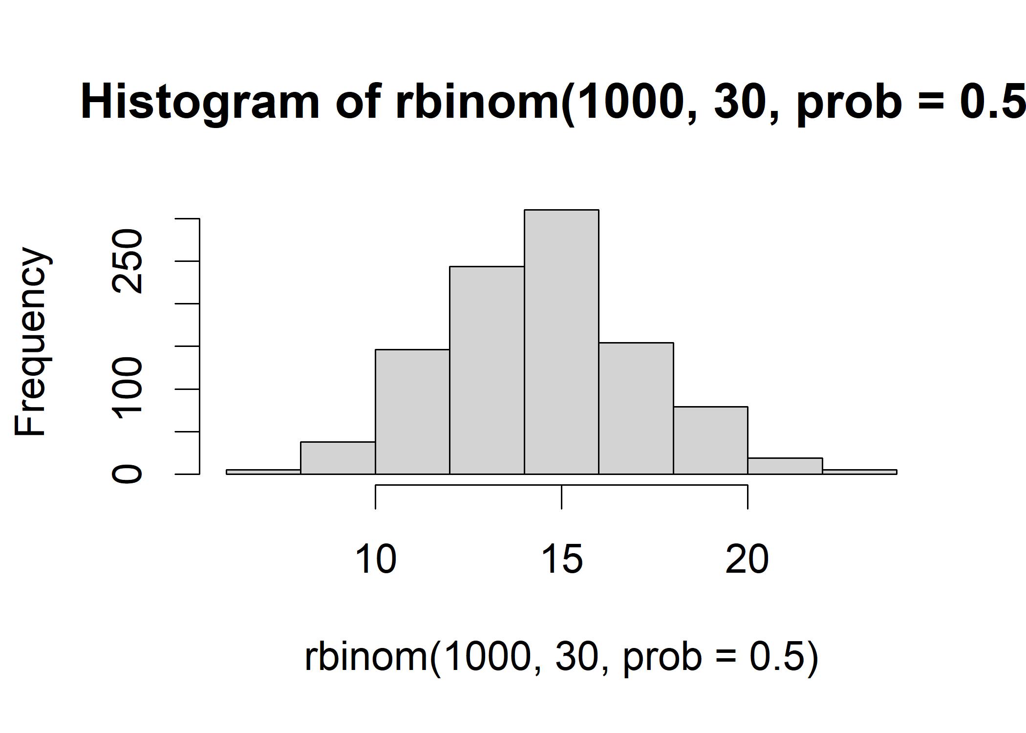 We then create a 2x2 contingency table with the jelly-down distribution follow the above binomial distribution.
set.seed(12)
# This table represents the null hypothesis of independence
expectedValues <- matrix(c(15,15,35,35), nrow=2, ncol=2, byrow=TRUE)
chiDist <- replicate(100000, calcChiSquared(make2x2table(rbinom(n=1, size=30,prob=0.5)),
                                            expectedValues))
hist(chiDist)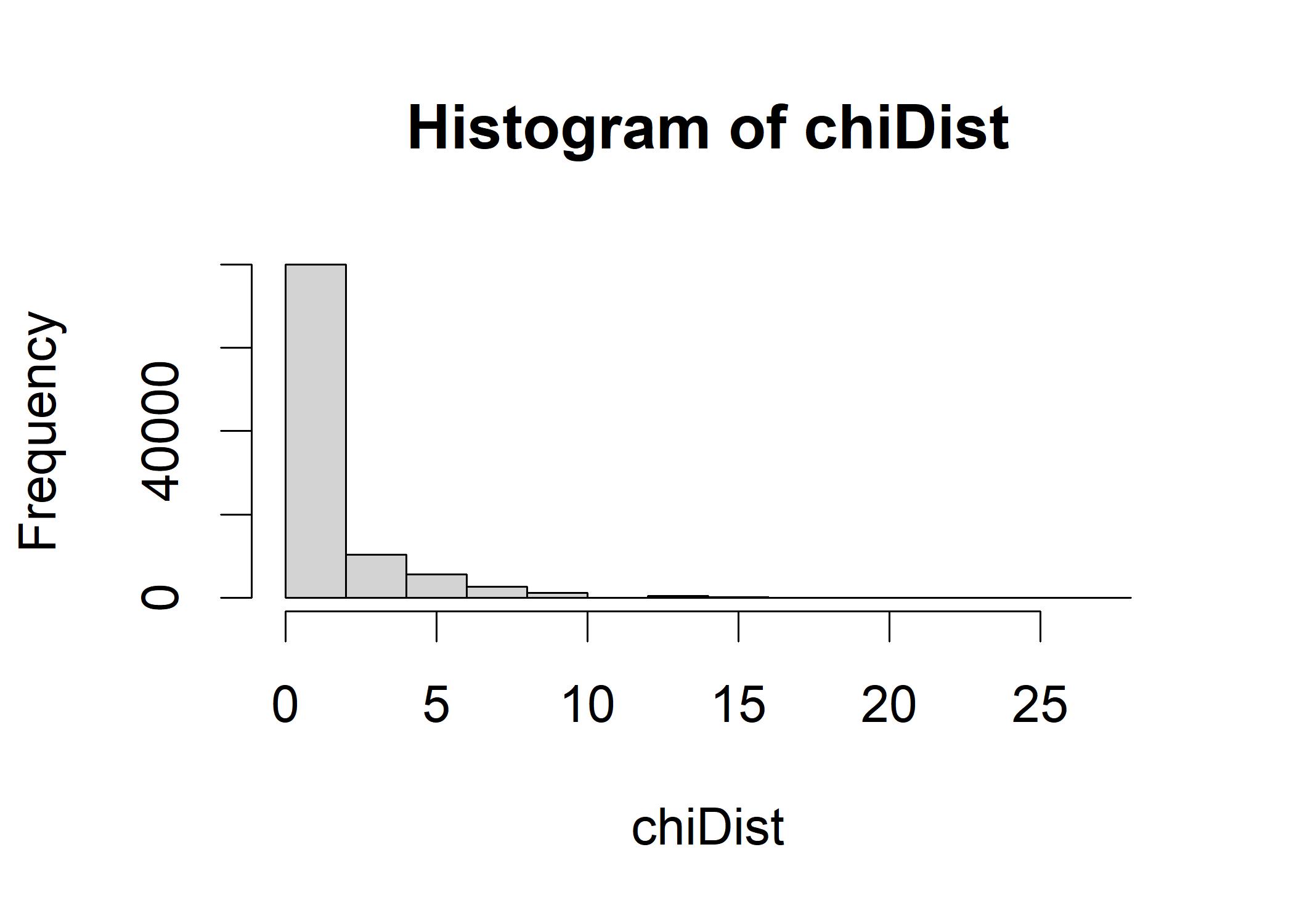
quantile(chiDist, probs=c(0.95))
##      95%
## 4.761905
The quantile suggests that any chi-square value greater than 4.76 is unlikely to be usual if the null hypothesis is true. This 4.76, around 5 means that if we make2x2table(15-5) and make2x2table(15+5) (in the following r chunk) will produce the same chi-square value. If we generate the jelly-down value more than 4.76, the chi-square value will be right on the threshold of the tail of the empirical distribution of chis-square in the above histogram.
# Yates correction, which would have made the chi- square test more conservative
# for small samples. Only use correct=TRUE if any one of the cells in the contingency
# table has fewer than five observations.
chisq.test(make2x2table(20), correct=FALSE)
##
##  Pearson's Chi-squared test
##
## data:  make2x2table(20)
## X-squared = 4.7619, df = 1, p-value = 0.0291
6.3.1 Bayesian Reasoning about Chi-Square Test
The Bayesian approach to infer the association between two categorical variables is to use the posterior distribution of the correlation. The contingencyTableBF() has four setting:
- “sampleType=poisson”: no special plans for the marginal proportions or total cases
- “sampleType=jointMulti”: total number is fixed
- “sampleType=indepMulti”: marginal proportions for either row or the column are fixed
- “sampleType=hypergeom”: marginal proportions for both row and the column are fixed
Let’s apply the Bayesian contingency test to the original toast-drop data.
library(BayesFactor)
ctBFout <- contingencyTableBF(make2x2table(20), sampleType="poisson", posterior=FALSE)
ctBFout
## Bayes factor analysis
## --------------
## [1] Non-indep. (a=1) : 4.62125 ±0%
##
## Against denominator:
##   Null, independence, a = 1
## ---
## Bayes factor type: BFcontingencyTable, poisson
The Bayes factor is 4.62, which is very strong evidence against the null hypothesis.
ctMCMCout <- contingencyTableBF(make2x2table(20), sampleType="poisson",
                                posterior=TRUE, iterations=10000)
summary(ctMCMCout)
##
## Iterations = 1:10000
## Thinning interval = 1
## Number of chains = 1
## Sample size per chain = 10000
##
## 1. Empirical mean and standard deviation for each variable,
##    plus standard error of the mean:
##
##              Mean    SD Naive SE Time-series SE
## lambda[1,1] 20.13 4.378  0.04378        0.04378
## lambda[2,1] 29.76 5.308  0.05308        0.05219
## lambda[1,2] 10.60 3.180  0.03180        0.03180
## lambda[2,2] 39.36 6.159  0.06159        0.06159
##
## 2. Quantiles for each variable:
##
##               2.5%    25%   50%   75% 97.5%
## lambda[1,1] 12.439 17.092 19.80 22.83 29.72
## lambda[2,1] 20.093 26.062 29.47 33.19 40.86
## lambda[1,2]  5.299  8.321 10.28 12.49 17.77
## lambda[2,2] 28.347 35.014 38.96 43.41 52.29
By looking at the posterior distribution of the correlation, we can see 95% HDI shows that the butter-down count range from 20.09 to 40.86. Let’s use the posterior distribution to create ratio of cell counts: jelly/butter for down-facing toast:
downProp <- ctMCMCout[,"lambda[1,1]"] / ctMCMCout[,"lambda[2,1]"]
hist(downProp)
The mean of this figure is around 0.667.
For the second column, we can calculate the ratio of cell counts: jelly/butter for up-facing toast:
The mean of this figure is around 0.667.
For the second column, we can calculate the ratio of cell counts: jelly/butter for up-facing toast:
upProp <- ctMCMCout[,"lambda[1,2]"] / ctMCMCout[,"lambda[2,2]"]
hist(upProp)
Now we compare the distribution of the ratio of cell counts for down-facing toast and up-facing toast.
diffProp <- downProp - upProp
hist(diffProp)
abline(v=quantile(diffProp,c(0.025)), col="black") # Lower bound of 95% HDI
abline(v=quantile(diffProp,c(0.975)), col="black") # Upper bound of 95% HDI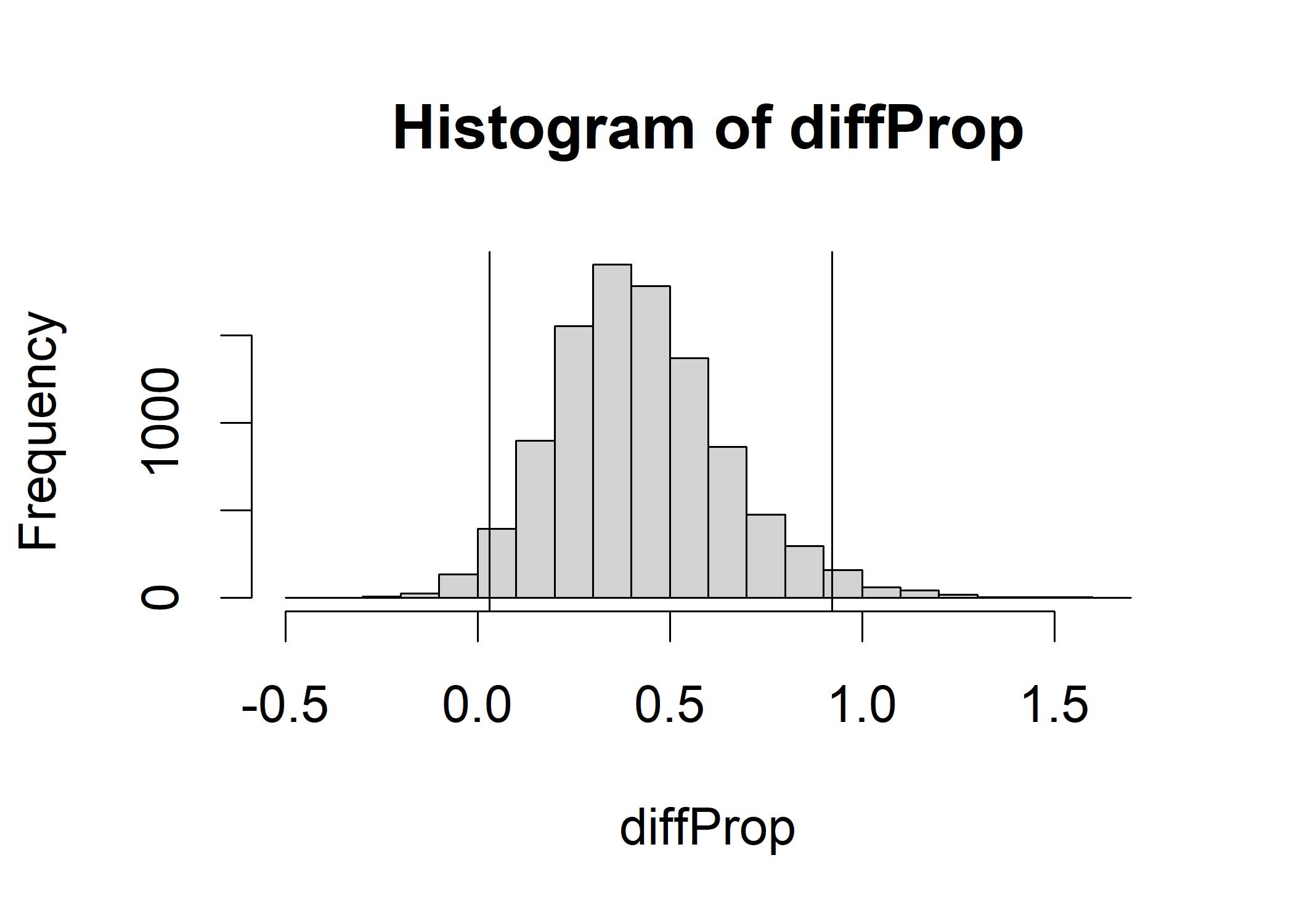 The histogram shows how much the jelly:butter ratio decreases as we switch from down-facing toast to up-facing toast.
The center is around 0.42, the 95% HDI is greater than 0 and less than 1, indicating we can reject the null hypothesis.
The histogram shows how much the jelly:butter ratio decreases as we switch from down-facing toast to up-facing toast.
The center is around 0.42, the 95% HDI is greater than 0 and less than 1, indicating we can reject the null hypothesis.