7.1 Frequentist Approach of Multiple Regression
We create a linear combination of the three independent variables and random noise, and divide each of them by 2 to get the square root of 4 that ensures that the standard deviation of GPA will be approximately one.
set.seed(321)
hardwork <- rnorm(120)
basicsmarts <- rnorm(120)
curiosity <- rnorm(120)
randomnoise <- rnorm(120)
gpa <- hardwork/2 + basicsmarts/2 + curiosity/2 + randomnoise/2
sd(gpa)
## [1] 1.011214
plot(hardwork, gpa)
# a is the intercept, b is the slope
abline(a=0, b=0.56)
# the error of prediction for a particular point
arrows(min(hardwork),gpa[which.min(hardwork)],min(hardwork), min(hardwork)*0.56)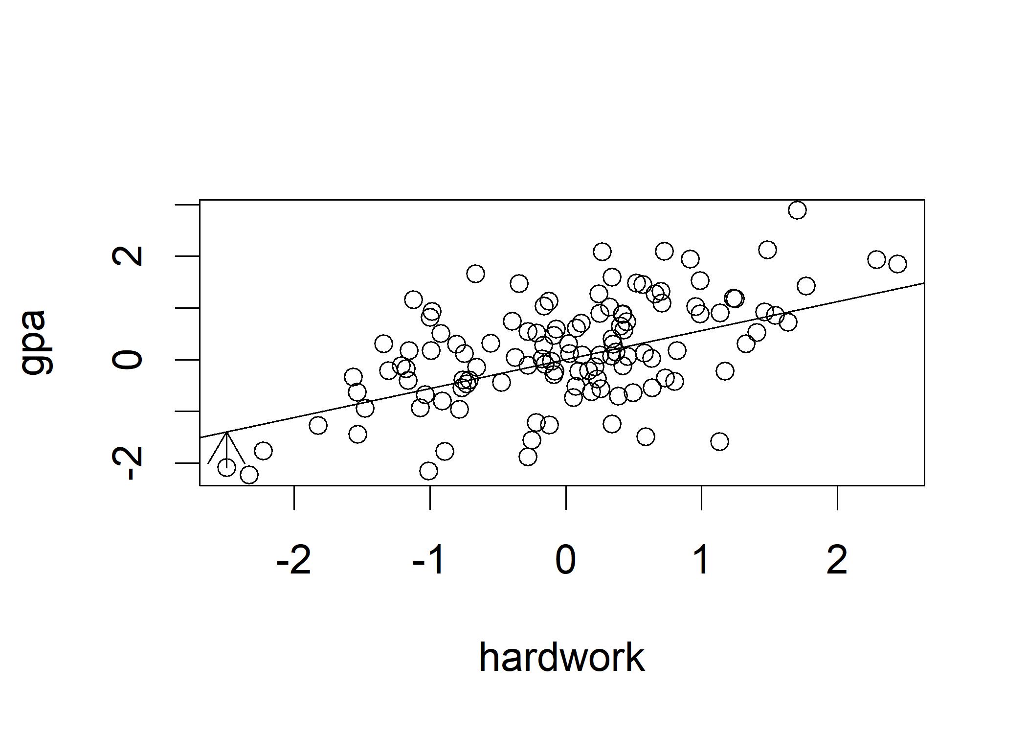 For visualization of bivariate, we use scatterplot where three elements are essential to look at:
- Linearity: If you can picture sketching a lovely straight line that roughly corresponds to the shape of the scatterplot’s point cloud, then the relationship between two variables will appear linear.
- Bivariate normality: points in the scatterplot will be a little bit denser close to the plot’s intersection point where the means of the X-axis and Y-axis variables overlap; Similarly, the scatterplot’s extreme points should appear sparser; linear multiple regression can be used to model nonnormal variables, but results must be evaluated with extra care.
- Influential outliers: One lone point in the far corner of the plot might have an excessive impact on the results of the study when using linear multiple regression because it is extremely sensitive to further outliers, especially at the high or low ends of the bivariate distributions.
From the figure we can observe that there is a line with the slope of around 0.56 fits the points and many of the points cluster around the point {0,0}. The arrow represents the error of prediction for that particular point. The error of prediction is calculated by the difference between the actual value and the prediction value. Now we plot errors of prediction for all the data points:
hist(gpa - (hardwork * 0.56))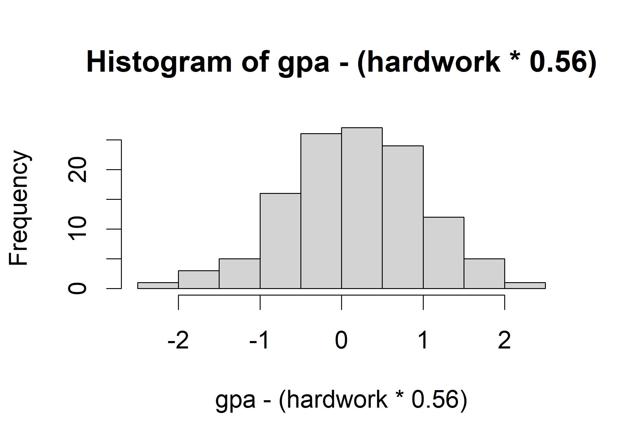
sum(gpa - (hardwork * 0.56))
## [1] 19.12997
The histogram shows that the errors of prediction are normally distributed. A lines fits perfectly all the points, then the errors ought to sum up to 0. However, if all the positive errors just cancel out all the negative ones, it might not be a good fit. So we might want to use the variance to get rid of the sign. Now we calculate the variance of the errors of prediction:
# dv = actual value of dependent variable, iv = value of independent variable
calcSQERR <- function(dv, iv, slope) {
(dv - (iv*slope))^2
}
head(calcSQERR(gpa, hardwork,0.56))
## [1] 3.742599e+00 8.443497e-06 2.959611e+00 1.432950e+00 1.451349e+00 3.742827e+00
sum(calcSQERR(gpa,hardwork,0.56))
## [1] 86.42242
hist(calcSQERR(gpa,hardwork,0.56))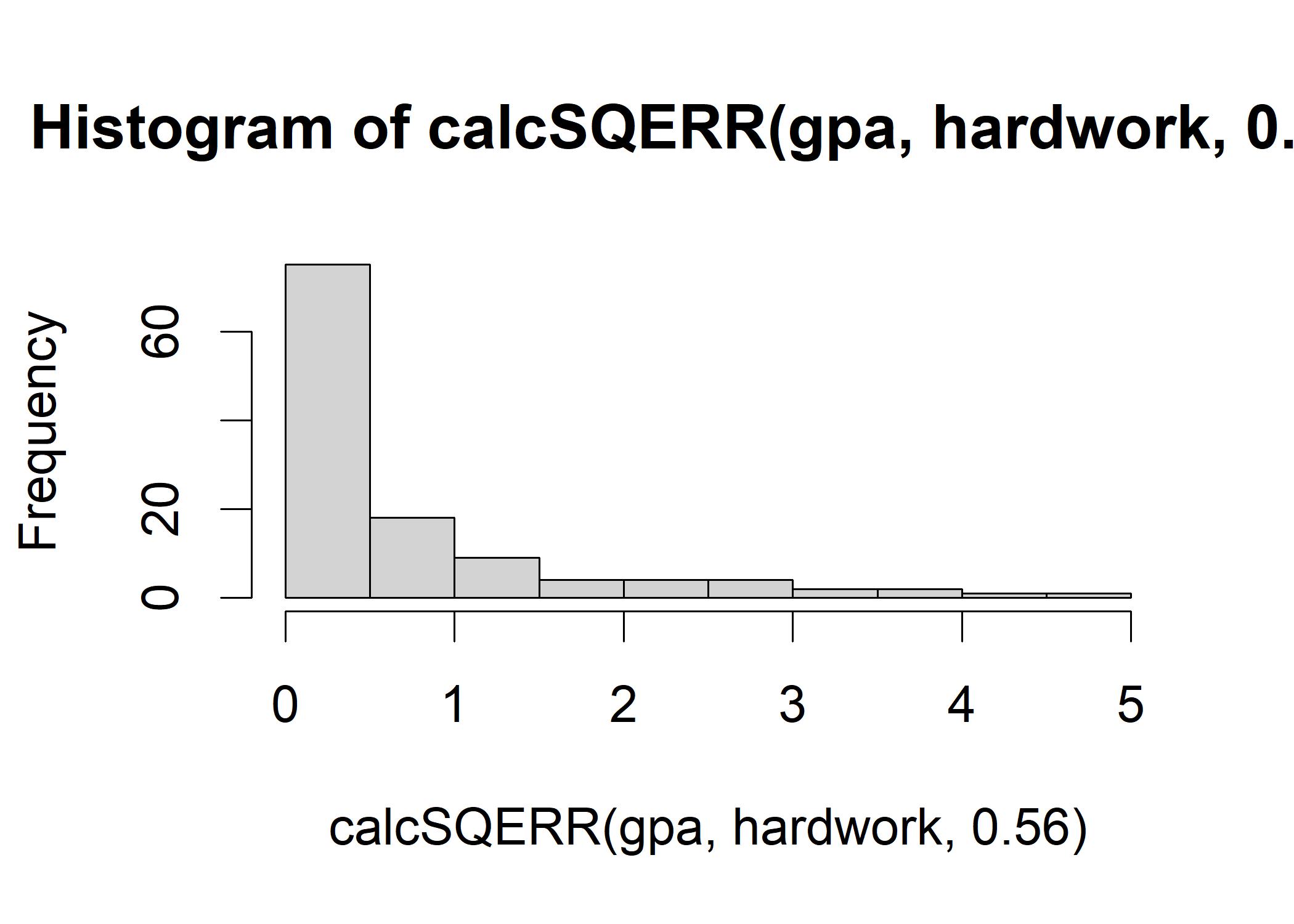 In this figure, most squared errors are small that near 0. We can apply a series of slope to test which one generates the smallest variance:
sumSQERR <- function(slope) {
sum(calcSQERR(gpa, hardwork, slope))
}
# create an evenly spaced sequence from 0 to 1, with 40 different values of slope to try out
trySlopes <- seq(from=0, to=1, length.out=40)
# sapply() # repeats calls to sumSQERR
sqerrList <- sapply(trySlopes, sumSQERR)
plot(trySlopes, sqerrList) # Plot the results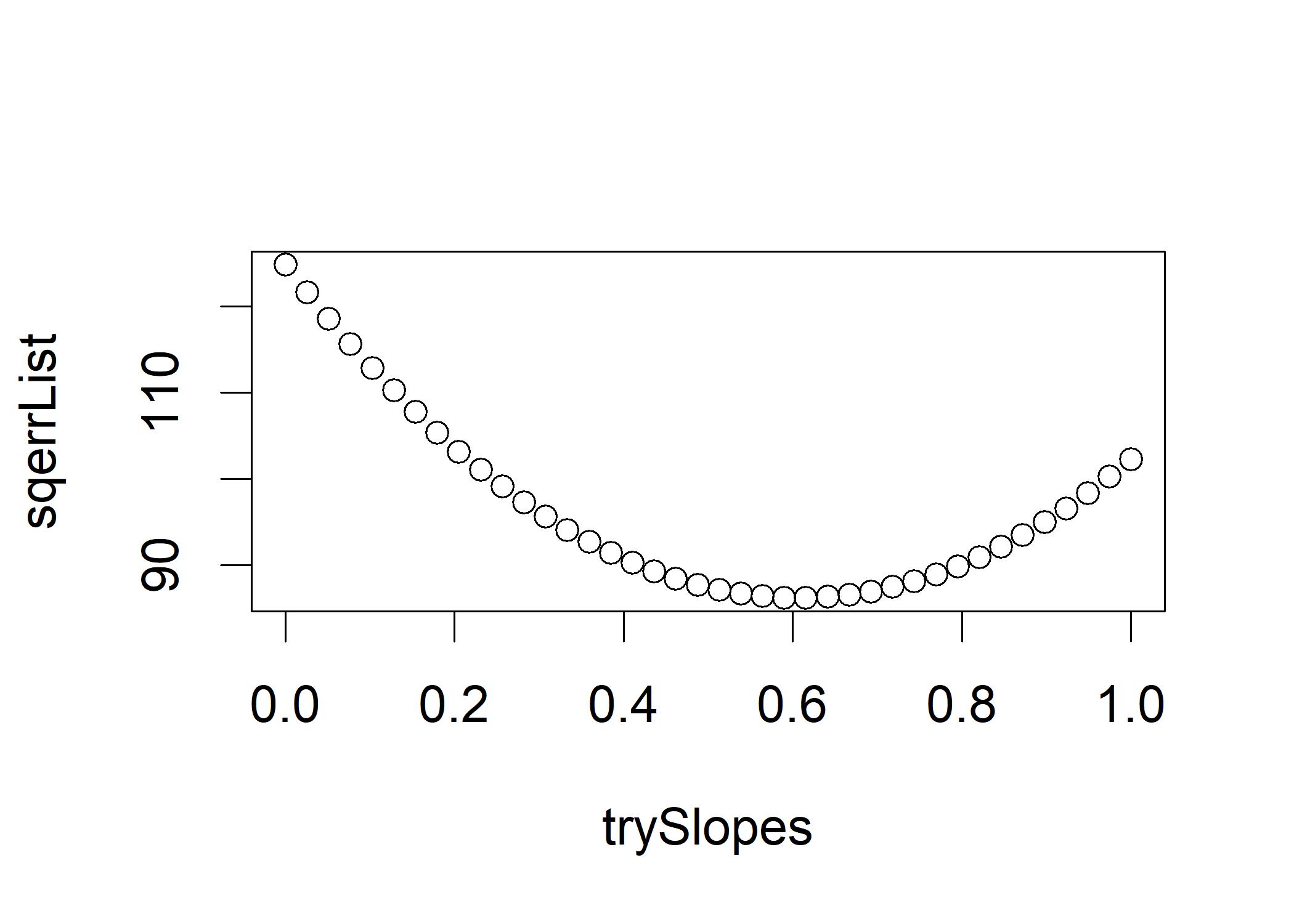 In this figure, a slope of 0 would represent no relationship between gpa and hardwork, and that the sum of the squared errors with a slope of 0 ought to be at a maximum.
A bivariate relationship’s best-fitting line is the one whose slope and intercept values, when combined and applied to all of the data points, minimize the sum of the squared errors of prediction.
Now, let’s use lm() to find the best-fitting line:
In this figure, a slope of 0 would represent no relationship between gpa and hardwork, and that the sum of the squared errors with a slope of 0 ought to be at a maximum.
A bivariate relationship’s best-fitting line is the one whose slope and intercept values, when combined and applied to all of the data points, minimize the sum of the squared errors of prediction.
Now, let’s use lm() to find the best-fitting line:
# Put everything in a data frame first
educdata <- data.frame(gpa, hardwork, basicsmarts, curiosity)
regOut <- lm(gpa ~ hardwork, data=educdata)  # Predict gpa with hardwork
summary(regOut) # Show regression results
##
## Call:
## lm(formula = gpa ~ hardwork, data = educdata)
##
## Residuals:
##      Min       1Q   Median       3Q      Max
## -2.43563 -0.47586  0.00028  0.48830  1.90546
##
## Coefficients:
##             Estimate Std. Error t value Pr(>|t|)
## (Intercept)  0.15920    0.07663   2.078   0.0399 *
## hardwork     0.60700    0.08207   7.396 2.23e-11 ***
## ---
## Signif. codes:  0 '***' 0.001 '**' 0.01 '*' 0.05 '.' 0.1 ' ' 1
##
## Residual standard error: 0.8394 on 118 degrees of freedom
## Multiple R-squared:  0.3167, Adjusted R-squared:  0.311
## F-statistic:  54.7 on 1 and 118 DF,  p-value: 2.227e-11
The summary of residuals gives an overview of the errors of prediction. The fact that the median is almost exactly 0 indicates that the residuals are symmetrically distributed, as they should be, and that there is no skewness in the residuals.
The coefficients section tell us the intercept in the first line and the slope in the second line. The standard errors around the estimates of slope and intercept show the estimated spread of the sampling distribution around these point estimates. The t-value demonstrates the Student’s t-test of the null hypothesis that each estimated coefficient is equal to zero. the R-squared value, which represents the effect size in a regression. This analysis’s multiple R-squared was just under 0.32, which indicates that hardwork accounted for roughly 32% of the variance in gpa.
In the last part, the standard error of the residuals is calculated by the sum-of- squared errors of prediction, dividing by the degrees of freedom, and taking the square root of the result. The F statistic that tests the null hypothesis that R-squared is equal to 0 is rejected.
In R we have 3D plots to show the best-fitting plane for three-dimensional cloud of points. Now let’s use three predictors.
regOut3 <- lm(gpa ~ hardwork + basicsmarts + curiosity, data=educdata)
summary(regOut3)
##
## Call:
## lm(formula = gpa ~ hardwork + basicsmarts + curiosity, data = educdata)
##
## Residuals:
##      Min       1Q   Median       3Q      Max
## -1.02063 -0.37301  0.00361  0.31639  1.32679
##
## Coefficients:
##             Estimate Std. Error t value Pr(>|t|)
## (Intercept)  0.08367    0.04575   1.829     0.07 .
## hardwork     0.56935    0.05011  11.361   <2e-16 ***
## basicsmarts  0.52791    0.04928  10.712   <2e-16 ***
## curiosity    0.51119    0.04363  11.715   <2e-16 ***
## ---
## Signif. codes:  0 '***' 0.001 '**' 0.01 '*' 0.05 '.' 0.1 ' ' 1
##
## Residual standard error: 0.4978 on 116 degrees of freedom
## Multiple R-squared:  0.7637, Adjusted R-squared:  0.7576
## F-statistic:   125 on 3 and 116 DF,  p-value: < 2.2e-16
In the coefficient part, we have three coefficients, aka. B-weights that are the slopes decribing the orientation of the best fitting hyperplane. The t-value demonstrates the Student’s t-test of the null hypothesis that each estimated coefficient is equal to zero. The multiple R-squared value of 0.76 in the model summary indicates that the three predictor variables jointly accounted for nearly three-quarters of the variance in gpa. There is an F-test (a null hypothesis significance test) of whether the multiple R-squared value is significantly different from 0.
The random noise that we injected mainly ended up in the residuals. When a set of residuals is notably nonnormal, it suggests that the relationship between the predictors and the dependent variable is not linear. there is an F-test (a null hypothesis significance test) of whether the multiple R-squared value is significantly different from 0.
plot(randomnoise, regOut3$residuals) The residuals from the regression analysis are almost perfectly correlated with the initial random noise variable.
But it is not perfect ball four of the variables are not entirely independent of each other.
The residuals from the regression analysis are almost perfectly correlated with the initial random noise variable.
But it is not perfect ball four of the variables are not entirely independent of each other.
cor(educdata)
##                   gpa   hardwork basicsmarts  curiosity
## gpa         1.0000000  0.5627970   0.5210660  0.3811908
## hardwork    0.5627970  1.0000000   0.2159194 -0.1356528
## basicsmarts 0.5210660  0.2159194   1.0000000 -0.1735183
## curiosity   0.3811908 -0.1356528  -0.1735183  1.0000000
The multiple linear regression examines the effect of one independent variable while controlling other independent variables. The slope/B-weights/coefficient only reflects its independent effect on the dependent variable.