Chapter 9 Logistic Regression
Both ANOVA and linear multiple regression belongs to general linear model we can use a mix of categorical and metric independent variables to predict metric dependent variable. In this chapter, we explore generalized linear model to create prediction model where dependent variable is categorical.
For general linear models, we use the least squares method to estimate the parameters. For generalized linear models, we use the maximum likelihood estimation to estimate the parameters. The maximum likelihood estimation is just for one point estimation while for Bayesian the posterior distribution is used to estimate the parameters.
We use inverse logit to predict binary outcomes.
# create X
logistX <- seq(from=-6, to=6, length.out=100)
# Compute the logit function using exp(), the inverse of log()
logistY <- exp(logistX)/(exp(logistX)+1)
plot(logistX,logistY)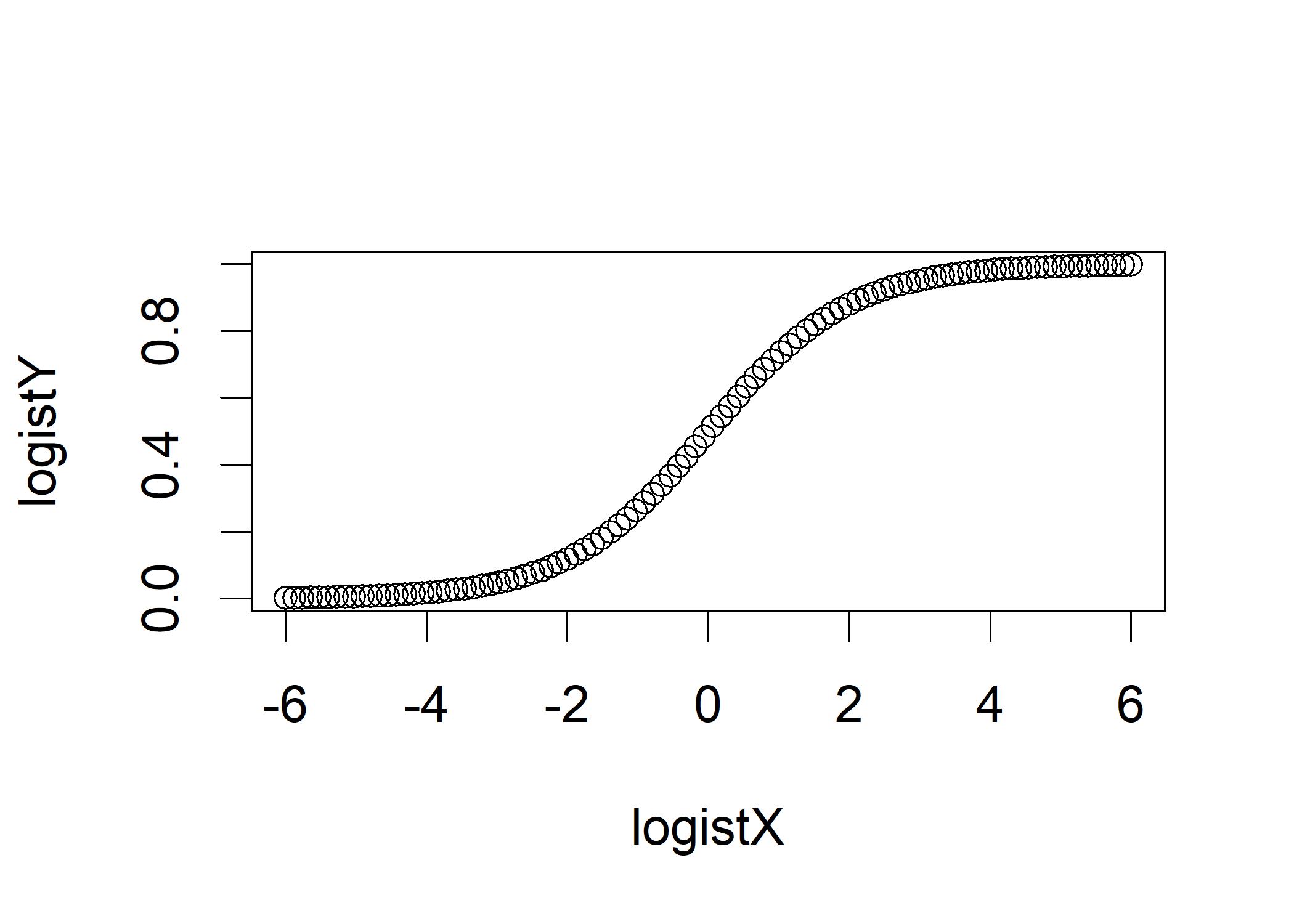 It is difficult to statistically model a step function, it is easier to model a continuous function such as the logit.
Now we create a random normal variable with mean of 0 and standard deviation of 1.
It is difficult to statistically model a step function, it is easier to model a continuous function such as the logit.
Now we create a random normal variable with mean of 0 and standard deviation of 1.
set.seed(123)
logistX <- rnorm(n=100,mean=0,sd=1)
logistY <- exp(logistX)/(exp(logistX)+1)
binomY <- round(logistY)
# Add noise to the predictor so that it does not perfectly predict the outcome
logistX <- logistX/1.41 + rnorm(n=100,mean=0,sd=1)/1.41
plot(logistX, binomY)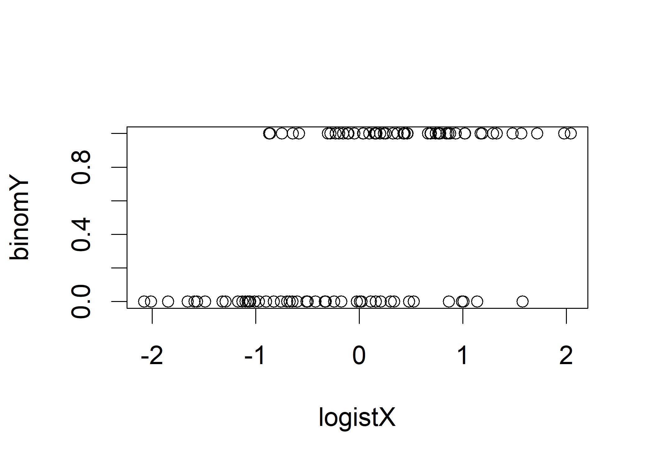 It is difficult to interpret the plot. We force the dichotomous Y variable into a factor with some friendly labels,
binomY <- factor(round(logistY), labels=c('Truth','Lie'))
logistDF <- data.frame(logistX, logistY, binomY) # Make data frame
boxplot(formula=logistX ~ binomY, data=logistDF, ylab="GSR", main="Lie Detection with GSR")
This plot can be interpreted as using truth/lie to predict GSR with ANOVA. Those truth has lower GSR than those lie. How good GSR in predicting truth/lie? We can use logistic regression to predict truth/lie from GSR.
# use binominal to invoke the invese logit
glmOut <- glm(binomY ~ logistX, data=logistDF, family=binomial())
summary(glmOut)
##
## Call:
## glm(formula = binomY ~ logistX, family = binomial(), data = logistDF)
##
## Deviance Residuals:
##     Min       1Q   Median       3Q      Max
## -2.3216  -0.7982   0.3050   0.8616   1.7414
##
## Coefficients:
##             Estimate Std. Error z value Pr(>|z|)
## (Intercept)   0.1199     0.2389   0.502    0.616
## logistX       1.5892     0.3403   4.671    3e-06 ***
## ---
## Signif. codes:  0 '***' 0.001 '**' 0.01 '*' 0.05 '.' 0.1 ' ' 1
##
## (Dispersion parameter for binomial family taken to be 1)
##
##     Null deviance: 138.47  on 99  degrees of freedom
## Residual deviance: 105.19  on 98  degrees of freedom
## AIC: 109.19
##
## Number of Fisher Scoring iterations: 4
The deviance residuals shows the distribution of the residuals after the model is fit. The p-value suggests that we reject the null hypothesis that the coefficient on logistX is 0 in the population. The coefficient for the linear regression is the slope of a line. However, the coefficient for logistic regression is the log odds ratio. The odds ratio is the ratio of the odds of the event to the odds of the non-event. The log-odds coefficient on our predictor is 1.5892. We can convert the log-odds to odds:
exp(coef(glmOut)) # Convert log odds to odds
## (Intercept)     logistX
##    1.127432    4.900041
This means if the GSR variable moved 1 unit, it is almost five times more likely that the subject is lying. The point estimate is a single estimate that may or may not be close to population value. We now look at the confidence interval around the estimate.
exp(confint(glmOut)) # Look at confidence intervals around log-odds
##                 2.5 %    97.5 %
## (Intercept) 0.7057482  1.812335
## logistX     2.6547544 10.190530
The intercept straddles 1:1, suggesting that the intercept is not statistically significant. 95% confidence interval for the logistX suggest that there is uncertainty around the point estimate of 4.9:1. The null deviance is the amount of error in the model if we assume that there is no connection between the X and Y variable. The residual deviance is how much the error in the null model is reduced by introducing the X variable. The difference between the null deviance and the model deviance is distributed as chi-square as:
anova(glmOut, test="Chisq") # Compare null model to one predictor model
## Analysis of Deviance Table
##
## Model: binomial, link: logit
##
## Response: binomY
##
## Terms added sequentially (first to last)
##
##
##         Df Deviance Resid. Df Resid. Dev  Pr(>Chi)
## NULL                       99     138.47
## logistX  1   33.279        98     105.19 7.984e-09 ***
## ---
## Signif. codes:  0 '***' 0.001 '**' 0.01 '*' 0.05 '.' 0.1 ' ' 1
The p-value suggests that we reject the null hypothesis that introducing logistX into the model causes zero reduction of model error. The last line AIC is the Akaike information criterion. The AIC investigates the amount of error reduction that a model was able to achieve in relation to the number of parameters (i.e., predictors and their coefficients) that were required to do so. AIC is useful for comparing nonnested models. For example, suppose we ran a single GLM model and used the variables A, B, C, D, E, and F to predict Y. Then, using D, E, F, and G, we predicted Y in a second GLM run. The AIC for the first model would be compared to the AIC for the second model. The model with the lower AIC is the better model.
Now we compare our model outputs with the original data
par(mfrow=c(1,2)) # par() configures the plot area
plot(binomY, predict(glmOut),ylim=c(-4,4)) # Predicted values
plot(binomY, logistX,ylim=c(-4,4)) # Original data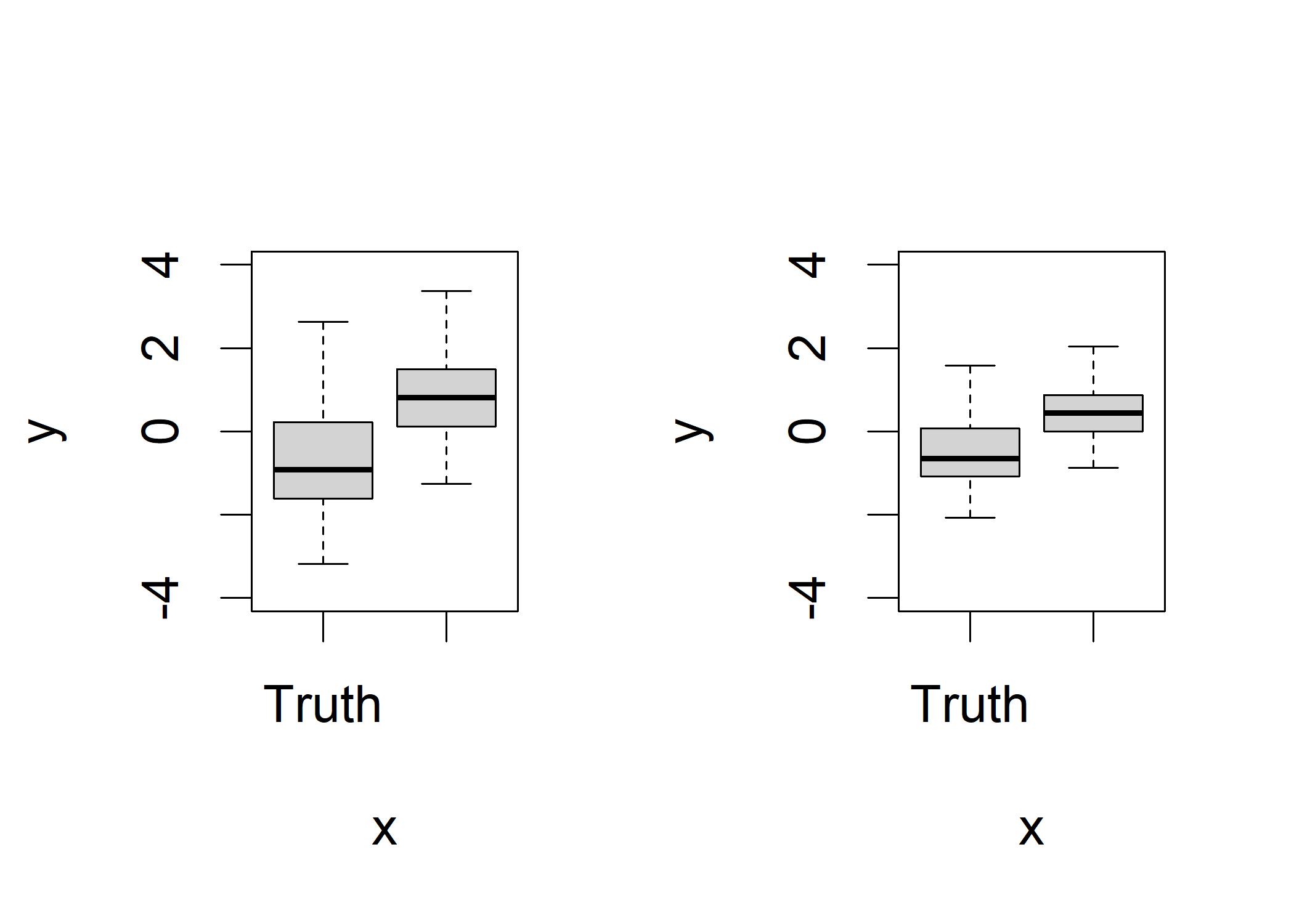 Observing the left plot, we can see that the X values for GSR are lower for truth than they are for liars.
It has larger variance compared to the right plot, which is caused by the natural effect of error that some of the X values are predicting the wrong thing in the prediction model.
Observing the left plot, we can see that the X values for GSR are lower for truth than they are for liars.
It has larger variance compared to the right plot, which is caused by the natural effect of error that some of the X values are predicting the wrong thing in the prediction model.