8.4 Bayesian Analysis of Regression Interactions

lmOutBayes1 <- lmBF(ozone ~ radiation + wind, data=stdenv)
lmOutBayes2 <- lmBF(ozone ~ radiation + wind + radiation:wind, data=stdenv)
lmOutBayes1
## Bayes factor analysis
## --------------
## [1] radiation + wind : 709773278516 ±0.01%
## 
## Against denominator:
##   Intercept only 
## ---
## Bayes factor type: BFlinearModel, JZS
lmOutBayes2
## Bayes factor analysis
## --------------
## [1] radiation + wind + radiation:wind : 4.272529e+12 ±0%
## 
## Against denominator:
##   Intercept only 
## ---
## Bayes factor type: BFlinearModel, JZS
lmOutBayes2/lmOutBayes1
## Bayes factor analysis
## --------------
## [1] radiation + wind + radiation:wind : 6.019568 ±0.01%
## 
## Against denominator:
##   ozone ~ radiation + wind 
## ---
## Bayes factor type: BFlinearModel, JZS

The Byes factor of the first model indicates that we favor the alternative hypothesis that the main effect of radiation and wind is not zero. The second model indicates that we favor the alternative hypothesis that the interaction term is not zero. The ratio of the two models indicates that we favor the model with interaction term.

mcmcOut <- lmBF(ozone ~ radiation + wind + radiation:wind, data=stdenv, posterior=TRUE, iterations=10000)
summary(mcmcOut)
## 
## Iterations = 1:10000
## Thinning interval = 1 
## Number of chains = 1 
## Sample size per chain = 10000 
## 
## 1. Empirical mean and standard deviation for each variable,
##    plus standard error of the mean:
## 
##                       Mean        SD  Naive SE Time-series SE
## mu                 0.01323  2.315529 2.316e-02      2.316e-02
## radiation          0.11794  0.026360 2.636e-04      2.696e-04
## wind              -5.15802  0.656880 6.569e-03      6.824e-03
## radiation.&.wind  -0.01956  0.007221 7.221e-05      7.221e-05
## sig2             596.64806 83.550790 8.355e-01      8.913e-01
## g                  0.51200  1.269399 1.269e-02      1.269e-02
## 
## 2. Quantiles for each variable:
## 
##                       2.5%       25%       50%       75%      97.5%
## mu                -4.50441  -1.53266   0.00737   1.54533   4.594048
## radiation          0.06517   0.10037   0.11845   0.13544   0.169603
## wind              -6.43385  -5.59661  -5.15912  -4.72258  -3.864110
## radiation.&.wind  -0.03376  -0.02446  -0.01953  -0.01473  -0.005593
## sig2             455.67202 537.25948 588.80715 648.32452 779.931667
## g                  0.07988   0.18007   0.29817   0.53584   2.095655

The 95% HDI for radiation, for wind and for their interaction does not include 0, which provide further evidence for the previous conclusion. Now we calculate the distribution of R-squared values.

rsqList <- 1 - (mcmcOut[,"sig2"] / var(stdenv$ozone))
mean(rsqList)    # Overall mean R- squared
## [1] 0.4611637
quantile(rsqList,c(0.025))
##      2.5% 
## 0.2956393
quantile(rsqList,c(0.975))
##   97.5% 
## 0.58848

The 95% HDI for R-squared ranges from 0.3 to 0.59. We can predict the outcomes.

# Set wind to a constant
loWind$wind <- mean(loWind$wind) - sd(loWind$wind)
hiWind$wind <- mean(hiWind$wind) + sd(hiWind$wind)
loWindOzone <- modelPredictions(lmOut1, Data=loWind, Type = 'response')
hiWindOzone <- modelPredictions(lmOut1, Data=hiWind, Type = 'response')
plot(loWind$radiation,loWindOzone$Predicted,xlim=c(0,350),ylim=c(10,90))
points(hiWind$radiation,hiWindOzone$Predicted,pch=3)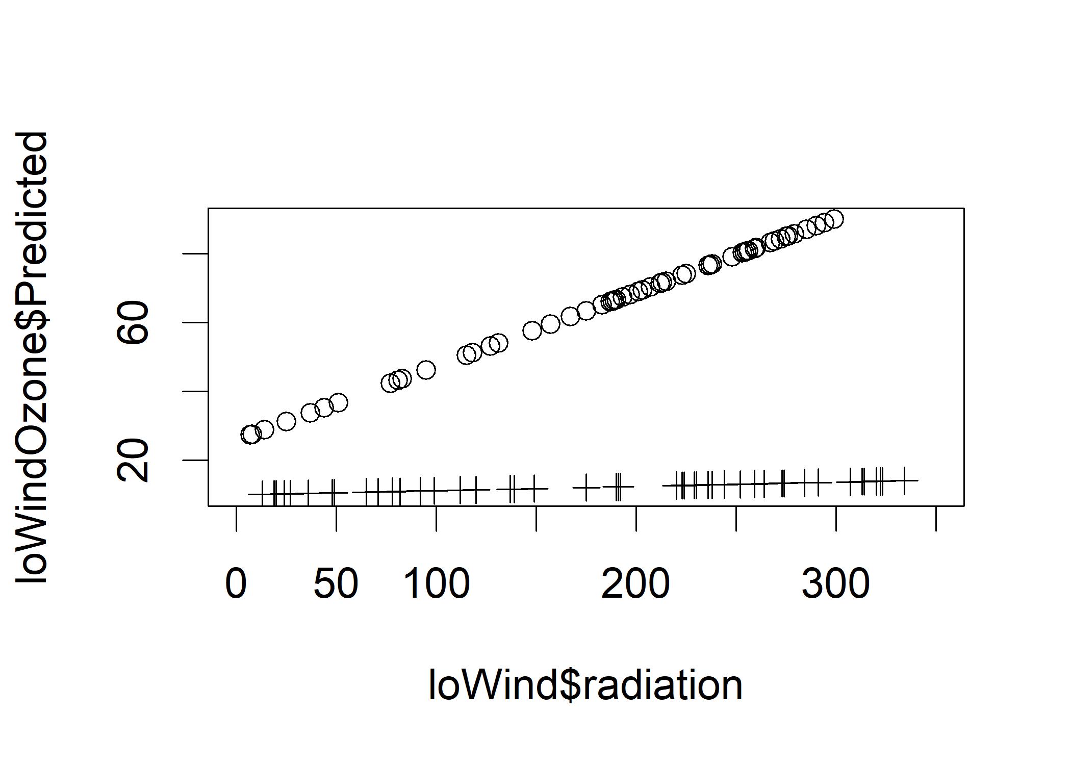

The circles are the predicted values for the low wind condition and the plus are the predicted values for the high wind condition. The line for the high wind condition shows minimal connection between radiation and ozone.