4.2 Markov chain Monte Carlo (MCMC)
MCMC consists of two processes including Markov chain and Monte Carlo. Markov chain is a stochastic process that satisfies the Markov property, which states that the future state of the process depends only on the present state and not on the history of the process. Mathematically, the Markov property can be expressed as \(P(X_{t+1} = x_{t+1} | X_{t} = x_{t}, X_{t-1} = x_{t-1}, \dots, X_{1} = x_{1}) = P(X_{t+1} = x_{t+1} | X_{t} = x_{t})\). Monte Carlo repeatedly samples from a known distribution (e.g., normal distribution) and computes some output from each sample (e.g., the sample mean). We process starting with a random candidate for the parameter we are modeling. In light of our data, we evaluate the posterior probability. After that, we slightly alter the parameter and reassess the posterior probability. We use a method of evaluation to compare these two probabilities, such as the Metropolis-Hastings approach, and then we decide whether to keep the parameter change based, in part, on whether the new parameter looks more likely. The parameter becomes our new “location” in the Markov chain if we keep it. We alter the parameter in a sequence of random moves that progressively create a whole distribution of likely parameter values by repeating this process thousands of times. In the end, we have a distribution of a set of parameter values.
Metropolis-Hastings
The M-H algorithms starts from a value \(\mathbf{x}\) of the generates the subsequent values \(x^t\) as follows:
- Generate a candidate value \(\mathbf{x}^{*}\) from a proposal distribution \(\pi(\mathbf{x}^{*}|\mathbf{x})\)
- compute the acceptance probabilty
- draw a uniform random number \(\mathbf{u}\) from the uniform distribution on [0,1]
- if \(\mathbf{u} < \alpha(\mathbf{x},\mathbf{x}^{*})\) then \(\mathbf{x}^{t+1} = \mathbf{x}^{*}\) else \(\mathbf{x}^{t+1} = \mathbf{x}\)
R illustration
This Bayesian t-test examined whether there was a mean difference in horsepower between manual and automatic transmission cars. Mean horsepower of manual transmission is 120.05, while mean horsepower of automatic transmission is 160.29. The Bayesian t-test produced a distribution of estimates for the mean difference. The center of this distribution was a difference of 40.2. The population mean difference probably lies somewhere close to this value: The 95% highest density interval for this distribution of estimates ranged from -18.3 to 98. 91.4% of the estimates are above zero and 8.6% are below zero. Among all the estimates generated, some of them overlap a mean difference of zero, thereby may suggest that there is no difference between the two groups.
library(BEST)
carsBest <- BESTmcmc(mtcars$hp[mtcars$am==0], mtcars$hp[mtcars$am==1])
carsBest
## MCMC fit results for BEST analysis:
## 100002 simulations saved.
## mean sd median HDIlo HDIup Rhat n.eff
## mu1 160.41 13.83 160.35 133.710 188.41 1.000 59603
## mu2 119.73 26.00 118.77 70.083 172.45 1.000 43285
## nu 31.27 28.84 22.49 1.056 88.72 1.003 15565
## sigma1 56.15 11.15 54.76 36.287 78.76 1.000 38149
## sigma2 84.04 24.73 81.37 36.524 134.93 1.000 22698
##
## 'HDIlo' and 'HDIup' are the limits of a 95% HDI credible interval.
## 'Rhat' is the potential scale reduction factor (at convergence, Rhat=1).
## 'n.eff' is a crude measure of effective sample size.
plot(carsBest)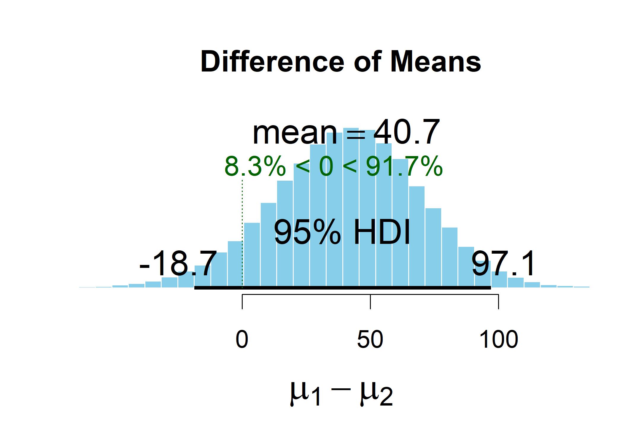 Looking into more details, we observe the information of carsBest.
- The rows represent the mean, standard deviation (SD), median, the lower bound of a highest density interval (HDI), the upper bound for an HDI, and
- The columns represent a population parameter for which we are seeking the posterior distribution.
- The effective form of each posterior distribution of means is shown by the symbol “nu” (Kruschke, 2013). An approximately normal distribution is indicated by higher values—generally speaking, any values greater than 30—while distributions with longer tails are indicated by lower values (and therefore more uncertainty).
- Rhat is a diagnostic value that, when it is close to 1.0, indicates that the MCMC process properly “converged” on reasonable findings. Values above 1.1 can point to an issue with the MCMC procedure that could be fixed by running extra stages.
- Effective sample size is abbreviated as n.eff. We do not count any of the steps that showed autocorrelation toward the effective sample size even though the whole MCMC process required 100,002 steps. We would also like to increase the number of steps in the MCMC procedure if n.eff were to ever fall below 10,000 for one or more of the lines in the table.
- The left corner 17.147 is an estimated point of the mean population value of the fuel efficiency of the car with automatic transmissions. SD (0.97), median (17.15), HDIlo (15.27), and HDIup (19.11)—describe the distribution of the 100,002 estimates in the posterior distribution.
- The second row is the parallel results of the posterior distribution of the population mean of the manual transmission cars.
Looking into more details, we observe the information of carsBest.
- The rows represent the mean, standard deviation (SD), median, the lower bound of a highest density interval (HDI), the upper bound for an HDI, and
- The columns represent a population parameter for which we are seeking the posterior distribution.
- The effective form of each posterior distribution of means is shown by the symbol “nu” (Kruschke, 2013). An approximately normal distribution is indicated by higher values—generally speaking, any values greater than 30—while distributions with longer tails are indicated by lower values (and therefore more uncertainty).
- Rhat is a diagnostic value that, when it is close to 1.0, indicates that the MCMC process properly “converged” on reasonable findings. Values above 1.1 can point to an issue with the MCMC procedure that could be fixed by running extra stages.
- Effective sample size is abbreviated as n.eff. We do not count any of the steps that showed autocorrelation toward the effective sample size even though the whole MCMC process required 100,002 steps. We would also like to increase the number of steps in the MCMC procedure if n.eff were to ever fall below 10,000 for one or more of the lines in the table.
- The left corner 17.147 is an estimated point of the mean population value of the fuel efficiency of the car with automatic transmissions. SD (0.97), median (17.15), HDIlo (15.27), and HDIup (19.11)—describe the distribution of the 100,002 estimates in the posterior distribution.
- The second row is the parallel results of the posterior distribution of the population mean of the manual transmission cars.